Gradient descent
algorithms gradient descent machine learning newton method optimizationContents
- Introduction
- Connection to Taylor series
- The Hessian matrix
- Newton optimization method
- Saddle points are sad
- References
Introduction
Gradient descent is an optimization algorithm for minimizing the value of a function. In the context of machine learning, we typically define some cost (or loss) function \(J(\boldsymbol{\theta})\) that informs us how well the model fits our data and \(\boldsymbol{\theta} = (\theta_0, \theta_1, \ldots)\) are the model’s parameters that we want to tune (e.g. the weights in a neural network or simply the coefficients in a linear regression problem of the form \(y = \theta_0 + \theta_1 x\)). The update rule for these parameters is:
\[\theta_j \leftarrow \theta_j - \alpha \frac{\partial}{\partial \theta_j} J(\boldsymbol{\theta})\]The symbol “\(\leftarrow\)” means that the variable to the left is assigned the value of the right side and \(\alpha\) is the learning rate (how fast we update our model parameters or how big steps we take when we change the values of the model’s parameters). The algorithm is iterative and stops when convergence is achieved, i.e. when the gradient is so small that \(\boldsymbol{\theta}\) doesn’t change.
This introduction is invariably accompanied by an image like this:
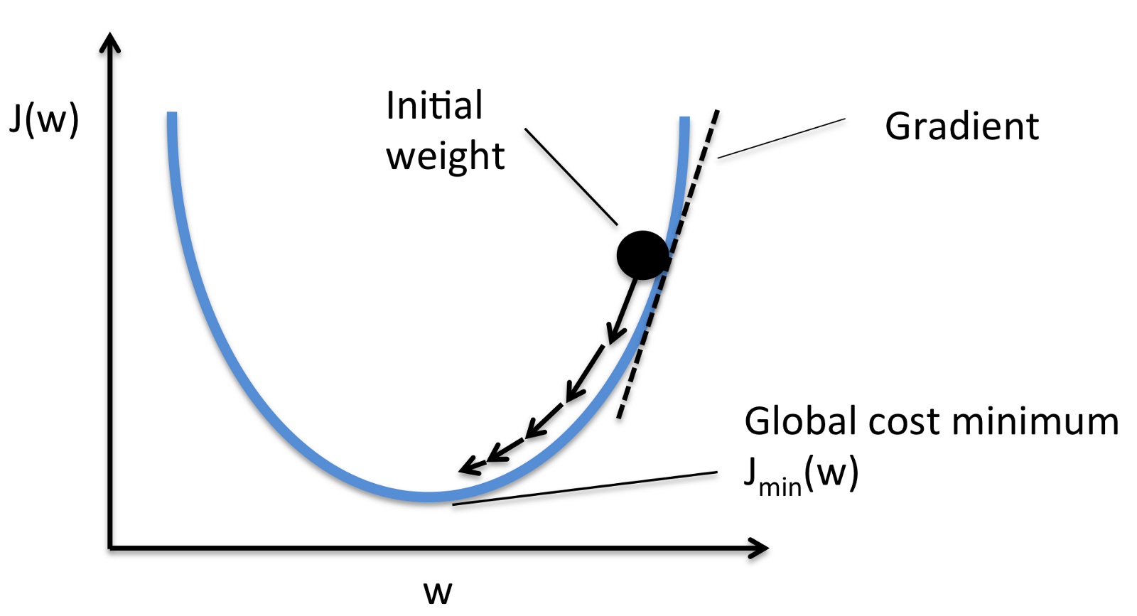
In the above scenario we only have \(1\) parameter, \(w\), and we want to minimize the cost function \(J(w)\). The intuition is that the sign of the gradient points us to the direction we have to move in order to minimize \(J\). Imagine that we have many parameters, then we are navigating inside a \(D-\)dimensional space. But since it’s easier to visualize with \(D=1\) or \(D=2\), most people use the above image as an example (or a 2D version of it).
Although the post is not about implementing gradient descent per se, let’s just take on a really simple example. Suppose we have some data in the form \((x_i,y_i)\) and we’d like to fit the linear regression model \(y = \theta_0 + \theta_1 x\).
ClearAll["Global`*"];
(* Generate some points along the y = 5x + 7 line plus some noise *)
data = Table[{x + RandomReal[], 7 + 5 x + RandomReal[]}, {x, 0, 10, 0.1}];
(* Define our cost function as the mean of the square error. Subscripting variables
doesn't work quite well, so let's just use u for theta0 and v for theta1.
J(u, v) = (1/n) * Sum (y_predicted - y_true)^2 *)
cost[u_, v_] := Mean[(u + v*First@# - Last@#)^2 & /@ data]
(* Set the learning rate and iterate for 1000 steps, initialize our estimates
of u,v and use gradient descent to update u,v *)
a = 10^-2;
costs =
Reap[
u = 0; v = 0;
For[i = 1, i <= 1000, i++,
u = u - a*D[cost[w0, w1], w0] /. {w0 -> u, w1 -> v};
v = v - a*D[cost[w0, w1], w1] /. {w0 -> u, w1 -> v};
Sow[cost[u, v]]
]
][[2, 1]];
(* Plot the function of cost J vs. iterations in both linear and log scale *)
Style[Grid[{
#[costs, Joined -> True, Filling -> Axis,
Frame -> {True, True, False, False},
FrameLabel -> {"Iterations", "Cost function J"},
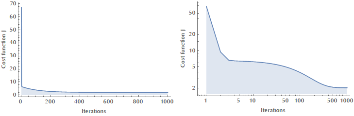
PlotRange -> All] & /@ {ListPlot, ListLogPlot}}],
ImageSizeMultipliers -> 1]This is how the cost function \(J(\theta_0, \theta_1)\) is reduced as we iterate (in the code above we write \(J(u, v)\) because subscripting isn’t so robust in Mathematica).
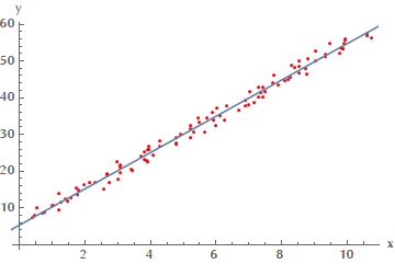
And this is our estimated linear model vs. our training data.
I’d like to present the same subject from a slightly different perspective, though, that doesn’t receive much attention.
Connection to Taylor series
Recall that a multivariable function \(f(\mathbf{x})\) can be written as a Taylor series:
\[f(\mathbf{x}+\delta \boldsymbol{x}) = f(\mathbf{x}) + \nabla_x f(\mathbf{x})\delta \boldsymbol{x} + \mathcal{O}\left(\left\|\delta^2 \boldsymbol{x}\right\|\right)\]Suppose that we want to minimize \(f(\mathbf{x})\), by taking a step from \(\mathbf{x}\) to \(\mathbf{x} + \mathbf{\delta x}\). This means that we would like \(f(\mathbf{x} + \delta\mathbf{x})\) to be smaller than \(f(\mathbf{x})\). If we substitute the formula from the Taylor expansion of \(f(\mathbf{x} + \delta\mathbf{x})\), we get:
\[f(\mathbf{x}+\delta \boldsymbol{x}) < f(\mathbf{x}) \Leftrightarrow f(\mathbf{x}) + \nabla_x f(\mathbf{x})\delta \boldsymbol{x} < f(\mathbf{x}) \Leftrightarrow \nabla_x f(\mathbf{x})\delta \boldsymbol{x} < 0\]To restate our problem: what is the optimal \(\delta\mathbf{x}\) step that we need to take so that the quantity \(\nabla_x f(\mathbf{x})\delta \boldsymbol{x}\) is minimized?
Keep in mind that \(\nabla_x f(\mathbf{x})\) and \(\delta \boldsymbol{x}\) are just vectors, therefore we need to minimize the dot product \(\mathbf{u} \cdot \mathbf{v}\), with \(\mathbf{u} = \nabla_x f(\mathbf{x})\) and \(\mathbf{v} = \delta \mathbf{x}\).
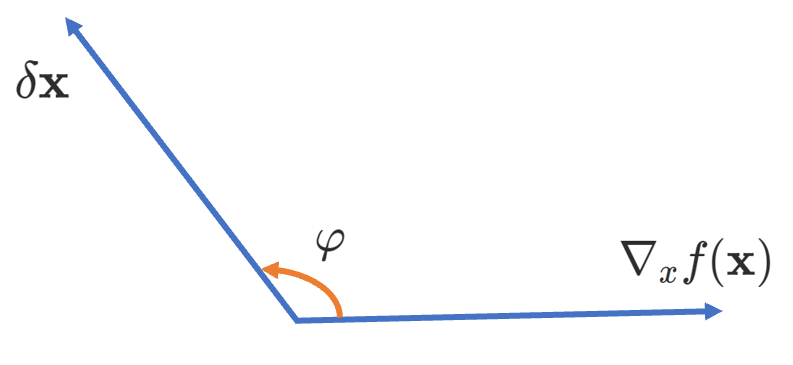
(To my fellow readers: sorry that \(\nabla f\) isn’t horizontal!)
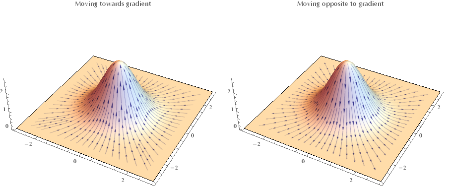
Since \(\mathbf{u} \cdot \mathbf{v} = \left\|u\right\| \left\|v\right\| \cos(\mathbf{u}, \mathbf{v})\) it follows that when the angle between \(\mathbf{u}\) and \(\mathbf{v}\) is \(\varphi = -\pi\), then the dot product takes its minimum value. Therefore \(\delta \mathbf{x} = - \nabla_x f(\mathbf{x})\). Keep in mind that this informs us only on the direction we have to travel in this multidimensional parameter space. The step size, i.e. how far we go along this direction in one step (iteration) is controlled by the learning rate \(\alpha\).
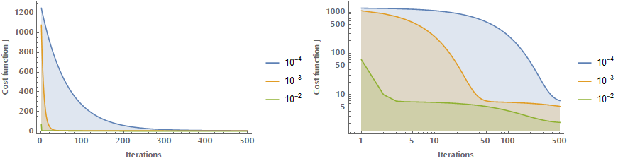
The following images illustrate the effect of different learning rates \(\alpha\) on the convergence. If \(\alpha\) is too small, we are converging too slow.
And if it’s too large, then we may be diverging!
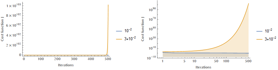
There’s a ton of literature on how to select optimal learning rates or how to change the learning rate during the optimization phase (google for adaptive learning rates, learning rate schedules and cyclical learning rates) but that’s beyond the scope of this introductory post.
The Hessian matrix
It’s interesting to consider what happens when the gradient becomes zero, i.e. \(\nabla_x f(\mathbf{x}) = 0\). Since it’s zero, this means that we are not moving towards any direction. At this point we have not yet assumed anything about the “shape” of the function, i.e. whether it was convex or non-convex. So, are we on a minimum? Are we on a saddle point?
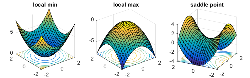
Image taken from here.
The answer to this question is hidden in the second-order terms of the Taylor series, which inform us about the local curvature in the neighborhood of \(\mathbf{x}\). Previously, when expanding \(f(\mathbf{x})\) we considered only the first-order terms. By also taking into account the second-order terms we get:
\[f(\mathbf{x}+\delta \boldsymbol{x}) = f(\mathbf{x}) + \nabla_x f(\mathbf{x})\delta \boldsymbol{x} + \frac{1}{2} \delta\mathbf{x}^T \mathbf{H}\delta\mathbf{x} + \mathcal{O}\left(\left\|\delta^3 \boldsymbol{x}\right\|\right)\]Where \(\mathbf{H} = \nabla_x^2f(\mathbf{x})\) is the Hessian matrix.
Now we are able to explore what’s happening in the case of \(\nabla_x f(\mathbf{x}) = 0\):
\[\begin{align} f(\mathbf{x}+\delta \boldsymbol{x}) &= f(\mathbf{x}) + \underbrace{\nabla_x f(\mathbf{x})\delta \boldsymbol{x}}_\text{zero} + \frac{1}{2} \delta\mathbf{x}^T \mathbf{H}\delta\mathbf{x} + \mathcal{O}\left(\left\|\delta^3 \boldsymbol{x}\right\|\right)\\ f(\mathbf{x}+\delta \boldsymbol{x}) &= f(\mathbf{x}) + \frac{1}{2} \delta\mathbf{x}^T \mathbf{H}\delta\mathbf{x} + \mathcal{O}\left(\left\|\delta^3 \boldsymbol{x}\right\|\right) \end{align}\]When the Hessian matrix is positive definite, by definition is \(\delta \mathbf{x}^T \mathbf{H} \delta \mathbf{x} > 0\) for any \(\delta \mathbf{x} \ne 0\). Therefore we have that \(f(\mathbf{x} + \delta\mathbf{x}) = f(\mathbf{x}) + (1/2) \delta\mathbf{x}^T \mathbf{H} f(\mathbf{x})\delta \mathbf{x} > f(\mathbf{x})\), which means that \(\mathbf{x}\) must be a local minimum. Similarly, when the Hessian matrix is negative definite, \(\mathbf{x}\) is a local maximum. Finally, when \(\mathbf{H}\) has both positive and negative eigenvalues, the point is a saddle point.
At this point we make a similar argument as before. We want to take a step from \(\mathbf{x}\) to \(\mathbf{x} + \mathbf{\delta x}\) and have \(f(\mathbf{x} + \delta\mathbf{x})\) be smaller than \(f(\mathbf{x})\). Therefore, we need to find a vector \(\delta \mathbf{x}\) for which \(\delta\mathbf{x}^T \mathbf{H} \delta \mathbf{x} < 0\) and move along it. How do we do that? I know that all these are too much of information, but bear with me a little more because things are about to get really interesting!
The Hessian matrix is given by \(\mathbf{H}f(x)_{(i,j)} = \frac{\partial^2}{\partial x_i\partial x_j}f(x)\). If the second partial derivatives are continuous, then the order of the differential operators \(\frac{\partial}{\partial x_i}\) and \(\frac{\partial}{\partial x_j}\) can be swapped. Which makes the Hessian matrix symmetric. Also \(\mathbf{H}\) is real-valued. We do know that in this case (real and symmetric) we may come up with and orthonormal basis \(e_1,…,e_n\), such that \(\mathbf{H}\) is written in the following diagonal form:
\[\mathbf{H} = \left( \array{\lambda_1 & 0 & \dots & 0 \\ 0 &\lambda_2 & 0 \dots & 0 \\ & & \dots & \\ 0 &\dots & 0 & \lambda_n } \right)\]If you choose for instance \(\delta \mathbf{x} = \mathbf{e}_i\) (that is, if you move along the direction of \(\mathbf{e}_i\)), then \(\delta \mathbf{x}^T \mathbf{H} \delta \mathbf{x} = \mathbf{e}_i^T \mathbf{H} \mathbf{e}_i = \mathbf{e}_i^T(\lambda_i \mathbf{e}_i)= \lambda_i \mathbf{e_i}^T \mathbf{e_i} = \lambda_i\), since \(e_i\) is an orthonormal basis. On the other hand if you choose some “random” direction \(\delta \mathbf{x}\) to move along, then this can be written as a linear combination of \(\mathbf{e}_i\): \(\delta \mathbf{x} = \sum_{i=1}^{N} x_i e_i\). Therefore:
\[\delta \mathbf{x}^T \mathbf{H} \delta \mathbf{x} = (e_1 x_1 \ldots e_n x_n) \left( \array{\lambda_1 & 0 & \dots & 0 \\ 0 &\lambda_2 & 0 \dots & 0 \\ & & \dots & \\ 0 &\dots & 0 & \lambda_n } \right) \left( \array{e_1 x_1 \\ \vdots \\ e_n x_n} \right) = \sum_{i=1}^{N} \lambda_i x_i^2\]What was all this fuzz about? We managed to write:
\[f(\mathbf{x} + \delta \mathbf{x}) = f(\mathbf{x}) + \frac{1}{2}\sum_{i=1}^N \lambda_i x_i^2\]This is very important because we expressed the value of \(f\) near \(\mathbf{x}\) as a sum of squares multiplied by the eigenvalues of \(\mathbf{H}\). If \(\mathbf{H}\) has only positive eigenvalues \(\lambda_i\) then for every \(\delta \mathbf{x}\) it’s \(f(\mathbf{x} + \delta \mathbf{x}) > f(\mathbf{x})\), i.e. we are on a local minimum. Because no matter what direction we take, the value of our function is increasing. Similarly we can show that if all the eigenvalues are negative, we are on a local maximum. Last, it becomes obvious that if \(\mathbf{H}\) has both positive and negative eigenvalues, we are sitting on a saddle point!
To sum up regarding the product \(\delta\mathbf{x}^T \mathbf{H} \delta \mathbf{x}\) we have these cases:
- \(\delta\mathbf{x}^T \mathbf{H} \delta \mathbf{x} > 0\): We are on a local minimum.
- \(\delta\mathbf{x}^T \mathbf{H} \delta \mathbf{x} < 0\): We are on a local maximum.
- \(\delta\mathbf{x}^T \mathbf{H} \delta \mathbf{x}\) has both positive and negative eigenvalues: We are on a saddle point.
- None of the above: We have no clue. We need even higher-order data to figure it out.
In case you feel that expressing \(f\) in terms of the Hessian matrix eigenvalues wasn’t rewarding enough, hold on! This analysis will help us have some insight on the scale of the learning rate \(\alpha\). Suppose we are on \(\mathbf{x}\) and we take a step \(\delta \mathbf{x} = - \alpha \nabla_x f(\mathbf{x})\). The value of our function at the new point \(\mathbf{x} - \alpha \nabla_x f(\mathbf{x})\) is:
\(f(\mathbf{x} - \alpha \nabla_x f(\mathbf{x})) = f(\mathbf{x}) - \alpha \nabla_x f(\mathbf{x})^T \nabla f(\mathbf{x}) + \frac{1}{2} \alpha^2 \nabla_x f(\mathbf{x})^T \nabla_x^2 f(\mathbf{x}) \nabla_x f(\mathbf{x}) + \mathcal{O}\left(\left\|\delta^3 \boldsymbol{x}\right\|\right)\).
For brevity let’s write \(\pmb{g} = \nabla_x f(\mathbf{x})\) and \(\mathbf{H} = \nabla_x^2 f(\mathbf{x})\), then:
\[f(\mathbf{x} - \alpha \pmb{g}) = f(\mathbf{x}) - \alpha \pmb{g^T} \pmb{g} + \frac{1}{2} \alpha^2 \pmb{g}^T \mathbf{H} \pmb{g}\]Ok, so what is the optimal step in terms of the learning rate \(\alpha_\text{opt}\)? Solve \(\nabla_\alpha f(\mathbf{x} - \alpha \pmb{g}) = 0\):
\[-\pmb{g}^T \pmb{g} + \alpha_\text{opt} \pmb{g}^T \mathbf{H} \pmb{g} = 0 \Leftrightarrow \alpha_\text{opt} = \frac{\pmb{g}^T \pmb{g}}{\pmb{g}^T \mathbf{H} \pmb{g}}\]Suppose we move along an eigenvector \(\mathbf{e}_i\), then:
\[\alpha_\text{opt} = \frac{\mathbf{e}_i^T \mathbf{e}_i}{\mathbf{e}_i^T \mathbf{H} \mathbf{e}_i} = \frac{1}{\mathbf{e}_i^T (\lambda_i \mathbf{e}_i)} = \frac{1}{\lambda_i}\]In the worst case scenario that we move along the eigenvector with the largest eigenvalue \(\lambda_\text{max}\), the optimal value for the learning rate \(\alpha\) is \(\frac{1}{\lambda_\text{max}}\). This analysis is valid to the extent that a quadratic function is a “good enough” approximation of \(f\) and gives as an idea on the scale of the learning rate \(a\).
Newton optimization method
As we’ve seen second-order terms in the Taylor expansion provide us with insights regarding the local curvature in the neighborhood of \(\mathbf{x}\). Naturally, we may ask whether we could come up with an optimization method that utilizes these information to converge faster (in less in steps). It turns out that this is what Newton method does.
\[f(\mathbf{x}+\delta \boldsymbol{x}) = f(\mathbf{x}) + \nabla_x f(\mathbf{x})\delta \boldsymbol{x} + \frac{1}{2} \delta\mathbf{x}^T \mathbf{H}\delta\mathbf{x} + \mathcal{O}\left(\left\|\delta^3 \boldsymbol{x}\right\|\right)\]The Newton method tries to find a step such that we end up in a stationary point (because if there is a minimum, it would reside on a stationary point). So, if we take the step to \(\mathbf{x} + \delta \mathbf{x}\) we would like this new point to be stationary:
\[\nabla_{\delta \mathbf{x}} f(\mathbf{x} + \delta\mathbf{x}) = 0\]The geometric interpretation of Newton’s method is that at each iteration, it fits a paraboloid to the surface of \(f(\mathbf{x})\) and then jumps into the maximum or minimum of that paraboloid (in higher dimensions, this may also be a saddle point). So the closer to quadratic our function looks at local level, the faster the convergence.
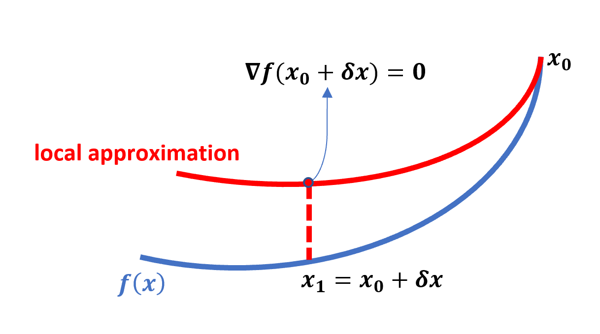
If we do the math and solve for \(\delta\mathbf{x}\) we get: \(\delta \mathbf{x} = -\mathbf{H}^{-1}\nabla f(\mathbf{x}) = - (\nabla^2 f(\mathbf{x}))^{-1} \nabla f(\mathbf{x})\) (obviously this only works if \(\mathbf{H}\) is invertible). Just as with gradient descent the best step that we could take to minimize \(f(\mathbf{x})\) was \(\delta \mathbf{x} = - \nabla_x f(\mathbf{x})\), for Newton method the best step is \(\delta \mathbf{x} = -\mathbf{H}^{-1}\nabla f(\mathbf{x})\).
Another derivation that I liked is the “linearized optimality condition” from the Book “Convex optimization” from Boyd, Section 9.5, page 485. Here, we linearize the optimality condition \(\nabla f(\mathbf{x} + \delta \mathbf{x}) = 0\):
\[\nabla f(\mathbf{x} + \delta \mathbf{x}) = \nabla f(\mathbf{x}) + \nabla^2 f(\mathbf{x}) \delta \mathbf{x} = 0 \Rightarrow \delta \mathbf{x} = -(\nabla^2 f(\mathbf{x}))^{-1}\nabla f(\mathbf{x})\]In practice we use \(\delta \mathbf{x} = -t\mathbf{H}^{-1}\nabla f(\mathbf{x})\). The optimal value of \(t\) is determined via the so called “backtracking line search”. In short, we start with \(t=1\) and while \(f(\mathbf{x} + t \delta \mathbf{x}) > f(\mathbf{x}) + \alpha t \nabla f(x)^T \delta\mathbf{x}\), we shrink \(t_\text{new} = \beta t_\text{old}\), else we perform the Newton update. It may puzzle you why the condition we are trying to satisfy (which by the way has a name, Armijo rule) is \(f(\mathbf{x} + t \delta \mathbf{x}) < f(\mathbf{x}) + \alpha t \nabla f(\mathbf{x})^T \delta\mathbf{x}\) and not just \(f(\mathbf{x} + t \delta \mathbf{x}) < f(\mathbf{x})\), but it turns out that we need to ensure a “sufficient” decrease of \(f(\mathbf{x})\). A decent descent!
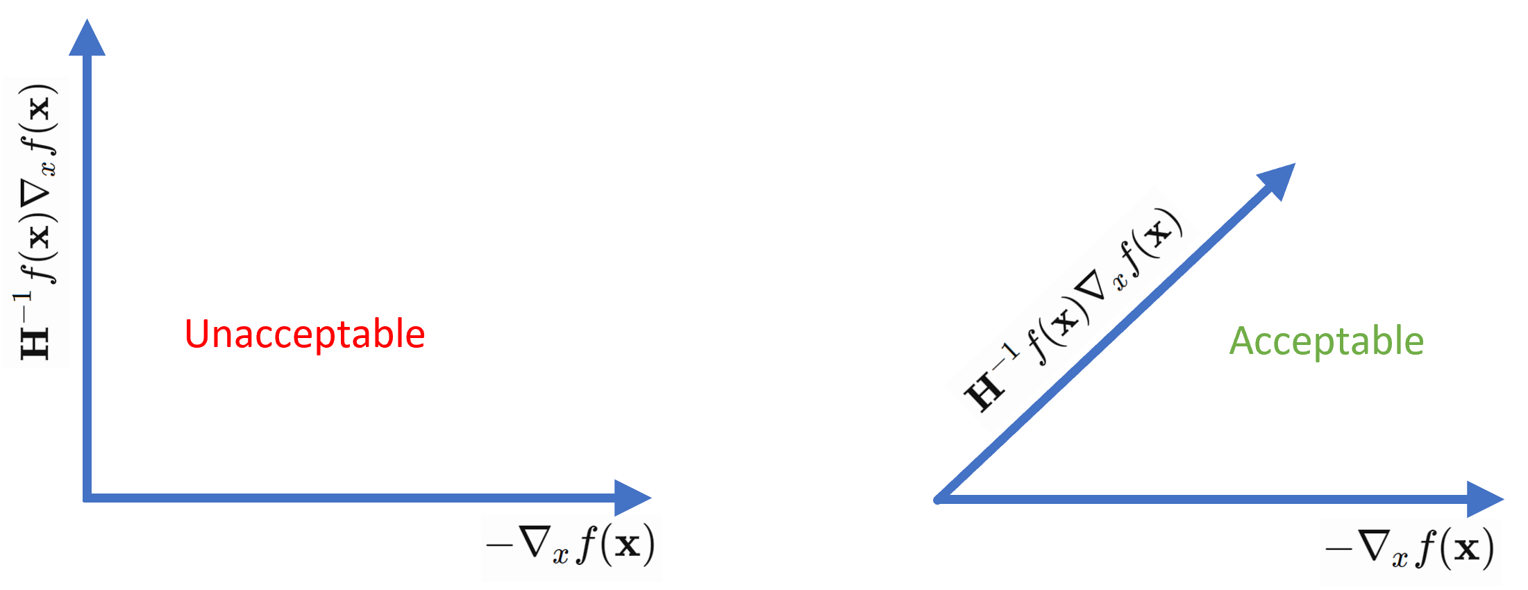
Last, the so called angle condition needs to be satisfied. The intuition is that we can’t be moving nearly orthogonal to the direction of gradient descent. Therefore we need the \(\cos(\mathbf{u}, \mathbf{v})\) to satisfy the condition \(\cos(\mathbf{u}, \mathbf{v}) \ge \epsilon > 0 \Leftrightarrow \frac{\mathbf{u} \cdot \mathbf{v}}{\left\| \mathbf{u} \cdot \mathbf{v} \right\|} \ge \epsilon\), where \(\mathbf{u} = \mathbf{H}^{-1}f(\mathbf{x}) \nabla_x f(\mathbf{x})\) and \(\mathbf{v} = -\nabla_x f(\mathbf{x})\).
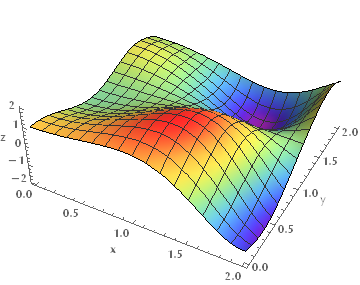
In the following images you can see how various optimization algorithms, including gradient descent and Newton’s method, perform on a simple minimization problem.
ClearAll["Global`*"];
<< Optimization`UnconstrainedProblems`
Plot3D[Cos[x^2 - 3 y] + Sin[x^2 + y^2], {x, 0, 2}, {y, 0, 2},
  ColorFunction -> "Rainbow", AxesLabel -> {"x", "y", "z"},
  Boxed -> False]
Style[
  Grid[
   Partition[#, 3]& [
    FindMinimumPlot[Cos[x^2 - 3 y] + Sin[x^2 + y^2], {{x, 1}, {y, 1}},
         Method -> #, PlotLabel -> #][[3]] & /@ {"Gradient", "Newton",
       "ConjugateGradient", "PrincipalAxis", "QuasiNewton",
      "InteriorPoint"}]],
  ImageSizeMultipliers -> 0.75
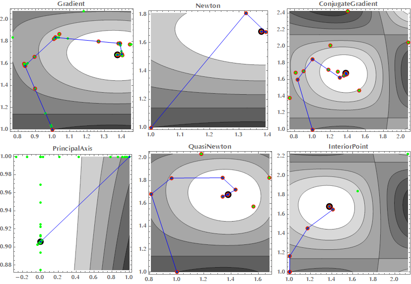
FindMinimumPlot runs FindMinimum, keeping track of the function and gradient calculations and steps taken during the search. The end image shows all these superimposed on a contour plot of the function. The steps are indicated with blue lines, function evaluations with green points and gradient evaluations with red points. The minimum found is shown with a large black point.
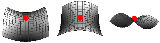
Saddle points are sad
In the early days of neural networks, it was believed that the proliferation of local minima would be a problem, in the sense that gradient descent would get stuck in them. But it turned out that this was not the case. Instead, the proliferation of saddle points, especially in high dimensional problems (e.g. neural networks), is usually the culprit (Dauphin et al, 2014). Such saddle points may be surrounded by plateaus where the error is high and they can dramatically slow down optimization, giving the impression that we are inside a local minimum.
For first-order optimization algorithms, such as gradient descent, it is not entirely clear how saddle points affect the optimization process. Near a saddle point, the gradient can often become very small. On the other hand, we do know empirically that gradient descent often manages to escape. It’s like leaving a ball on a surface with the shape of a saddle. At first the ball may stand still, but even the slightest perturbation will eventually make it roll and escape because this equilibrium is unstable.
ClearAll["Global`*"];
f[x_, y_] := x^2 - y^2
Style[Grid[{
   Table[
    Show[
     Plot3D[f[x, y], {x, -2, 2}, {y, -2, 2},
      ColorFunction -> GrayLevel, Boxed -> False,
      AxesLabel -> {"x", "y", "z"}, Axes -> False, ViewPoint -> d],
     Graphics3D[
      {Red, AbsolutePointSize[20], Point[{0, 0, 1.5}]}
      ]
     ],
    {d, {{0, 2, 2}, {2, 0, 2}, {2, 2, 0}}}]
   }], ImageSizeMultipliers -> 1/2]
For Newton’s method (in its standard form), saddle points clearly constitute a problem (Goodfellow, 2016). Gradient descent is designed to move “downhill”, whereas Newton’s method, is explicitly designed to search for a point where the gradient is zero (remember that we solved for \(\nabla f(\mathbf{x} + \delta \mathbf{x}) = 0\)). In its standard form, it can as well jump into a saddle point. In the example above we have \(f(x,y) = x^2 - y^2\), let’s calculate \((x,y)_{n+1} = (x,y)_{n} - \mathbf{H}^{-1}f(x,y) \nabla f(x, y)\):
ClearAll["Global`*"];
f[x_, y_] := x^2 - y^2
{x, y} - Inverse@D[f[x, y], {{x, y}, 2}] . Grad[f[x, y], {x, y}]
(* {0, 0} *)
Do you see how Newton method sent us to the saddle point?
The proliferation of saddle points in high-dimensional parameter spaces may explain why second-order methods have not replaced gradient descent in the context of neural network training. Another problem with Newton’s method is that although it usually takes less steps to converge, the computational burden of these steps is considerable (particularly the calculation of \(\mathbf{H}^{-1})\). To be fair though, there are modified versions of the Newton method, such as the “saddle free Newton” or methods that approximate \(\mathbf{H}\) to speed up computations.
References
- Dauphin Y, Pascanu R, Gulcehre C, Cho K, Ganguli S, Bengio Y. Identifying and attacking the saddle point problem in high-dimensional non-convex optimization [Internet]. arXiv [cs.LG]. 2014. Available from: http://arxiv.org/abs/1406.2572
- Goodfellow I, Bengio Y, Courville A. Deep Learning. MIT Press; 2016. 800 p.
- Unconstrained optimization book part1 and part2.