Norms and machine learning

Contents

• Introduction
• Norms
  • Properties
  • The \(\ell_p\) norm
• Connection with optimization
  • Regularization
  • Feature selection
  • Convexity of the norms

Introduction

A vector space, known also as a linear space, is a collection of objects (the vectors), which may be added together and multiplied by some scalar (a number). In machine learning we use vectors all the time. Here are some examples:

• Feature vectors are collections of numbers that we group them together when representing an object. In image processing, the features’ values may be the pixels of the image, so assuming a 128 \(\times\) 128 grayscale image, we get a 16384 long vector. Features are equivalent to independent variables (the \(x\)-s) in linear regression, but usually are more numerous.
• The output of a machine learning model, say a neural network that is trained to identify hand-written digits, may be represented as a vector, e.g. \(y = [0, 0, 1, 0, 0, 0, 0, 0, 0, 0]^T\) for representing “2” as the correct output. By the way this representation is called one hot encoding and the vector one hot vector :D
• The loss function, i.e. the function that tells us how good or how bad are predictions are, is also directly related to the norm of a particular vector space. For example, the mean squared error is defined as \(\text{MSE} = \frac{1}{N} \sum_i (y_{\text{true,}i} - y_{\text{predicted,}i})^2\), which (as we shall see) is connected to the \(\ell_2\) norm of vectors \(y_i = y_{\text{true,}i} - y_{\text{predicted,}i}\).
• The parameters of a model, say the weights of a neural network, can be thought as a long vector \(w\). This representation is useful when we apply regularization during the training of the network, so that we keep the coefficients of the model small (or, some of them, zero), preventing the model from becoming more complex than it ought to be.

Let’s see what does it mean for a vector space to have a norm.

Norms

Properties

Informally, a norm is a function that accepts as input a vector from our vector space \(V\) and spits out a real number that tells us how big that vector is. In order for a function to qualify as a norm, it must first fulfill some properties, so that the results of this metrization process kind of “make sense”. These properties are the following. For all \(u, v\) in the vector space \(V\) and \(\alpha\) in \(\mathbb{R}\):

• \(\|v\| \ge 0\) and \(\|v\| = 0 \Leftrightarrow v = 0\) (positive / definite)
• \(\| \alpha v \| = \|\alpha\| \| v \|\) (absolutely scalable)
• \(\|u+v\| \le \|u\|+\|v\|\) (triangle inequality)

The \(\ell_p\) norm

One of the most widely known family of norms is the \(\ell_p\) norm, which is defined as:

\[\ell_p = \left( \sum_{i=1}^N |x_i|^p \right)^{1/p}, \text{for } p \ge 1\]

For \(p = 1\), we get \(\ell_1 = \vert x_1 \vert + \vert x_2 \vert + \ldots + \vert x_n \vert\)

For \(p = 2\), \(\ell_2 = \sqrt{x_1^2 + x_2^2 + \ldots + x_n^2}\)

For \(p = 3\), \(\ell_3 = \sqrt[3]{\vert x_1 \vert ^3 + \vert x_2 \vert ^3 + \ldots + \vert x_n \vert ^3}\)

For \(p \to \infty\), \(\ell_\infty = \max_i (\vert x_1 \vert, \vert x_2 \vert, \ldots, \vert x_n \vert)\)

Every \(\ell_p\) assigns a different “size” to vectors and the answer to the question on what’s the best \(\ell_p\) norm to use, depends on the problem you are solving. For example, if you are building an application for taxi drivers in Manhattan that needs the minimal distance between two places, then using the \(\ell_1\) norm (purple) would make more sense than \(\ell_2\) (green). Because the \(\ell_2\) distance “is not accessible” to a taxi driver, as s/he can only navigate through the purple roads. But if the same app was meant to be used by helicopter pilots, then the green line would serve them better. Here I’m mixing the notions of norm (“length” or “size”) and metric (“distance”), but you get the idea.

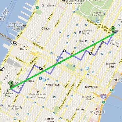
Image taken from quora.com.

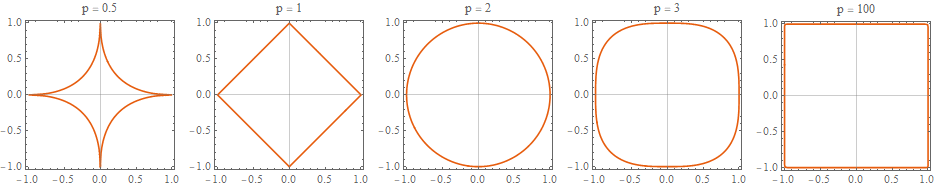
In the following image we can see the shape of the \(\ell_p\) norm for various values of \(p\). The vector space that we are operating is \(\mathbb{R}^2\). Concretely, we see the boundary of \(\ell_p = 1\), i.e. all those vectors \(v = (x,y)\) whose \(\ell_p\) norm equals \(1\).

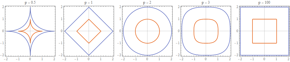
These are two boundaries for \(\ell_p = 1\) and \(\ell_p = 2\).

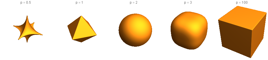
And this is the boundary for \(\ell_p = 1\) in \(\mathbb{R}^3\), that is the set of all \((x,y,z)\) points for which the vector \(v = (x,y,z)\) has an \(\ell_p\) equal to 1.

At this point the careful reader might have noticed that \(p\) should be a real number greater than or equal to 1. So is \(\ell_{1/2}\) really a norm? The answer is no, because it violates the triangle equality. Let \(v = (x_1, y_1), w = (x_2, y_2)\) then \(v+w=(x_1+x_2, y_1+y_2)\).

\[\|v+w\| \le \|v\|+\|w\| \Leftrightarrow \left(\sqrt{x_1+x_2} + \sqrt{y_1+y_2} \right)^2 \le \left(\sqrt{x_1} + \sqrt{y_1}\right)^2 + \left( \sqrt{x2} + \sqrt{y_2}\right)^2\]

If you expand the squares and simplify the inequality, you will end up in a false statement.

Connection with optimization

Let’s see two applications of norms in machine learning, namely regularization and feature selection. Though, the latter is merely a special form of regularization which, by design, favors the generation of sparse solutions.

Regularization

In statistical regression or machine learning, we regularly (:D) penalize either the \(\ell_1\) norm of a solution’s vector of parameter values or its \(\ell_2\). Techniques that use the former penalty, like LASSO, encourage solutions where many of model’s parameters are assigned to zero (as we shall see in a bit). Techniques which use an \(\ell_2\) penalty, like ridge regression, encourage solutions where most parameter values are small (but not necessarily zero). Elastic net regularization uses a penalty term that is a combination of the \(\ell_1\) norm and the \(\ell_2\) norm of the parameter vector.

Suppose that we are training a neural network model to read hand written digits and we are using a loss (or cost function) \(J\) (\(N\) is the number of training examples):

\[J = \text{MSE} = \frac{1}{N} \sum_{i=1}^N (y_i - \hat{y}_i)^2\]

We could add an \(\ell_1\) penalty term (\(m\) is the number of model’s parameters):

\[J = \underbrace{\frac{1}{N} \sum_{i=1}^N (y_i - \hat{y}_i)^2}_{\text{Mean Squared Error}} + \underbrace{\lambda \sum_{j=1}^m \vert w_j \vert}_{\lVert w\rVert_1 \text{ penalty}}\]

The hyperparameter \(\lambda\) is controlling how large penalty we impose on the cost function. If \(\lambda\) is large, then the model’s parameters \(w_j\) must be pushed towards zero, so that the product \(\lambda \lVert w \rVert_1\) is minimized. On the other hand, if \(\lambda\) is already small, then the penalty is relaxed.

Or we could add an \(\ell_2\) penalty term:

\[J = \underbrace{\frac{1}{N} \sum_{i=1}^N (y_i - \hat{y}_i)^2}_{\text{Mean Squared Error}} + \underbrace{\lambda \sum_{j=1}^m {\vert w_j \vert}^2}_{\lVert w \rVert_2^2 \text{ penalty}}\]

In elastic regularization, we use a combination of \(\ell_1\) and \(\ell_2\) penalty:

\[J = \underbrace{\frac{1}{N} \sum_{i=1}^N (y_i - \hat{y}_i)^2}_{\text{Mean Squared Error}} +\underbrace{\lambda \left[\alpha \sum_{j=1}^m {\vert w_j \vert} + (1-\alpha) \sum_{j=1}^m {\vert w_j \vert}^2 \right]}_{\text{Combined } \lVert w \rVert_1 \text { and } \lVert w \rVert_2^2}\]

With the hyperparameter \(\alpha \in [0,1]\) controlling how much of one versus the other we use in the mixing.

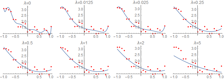
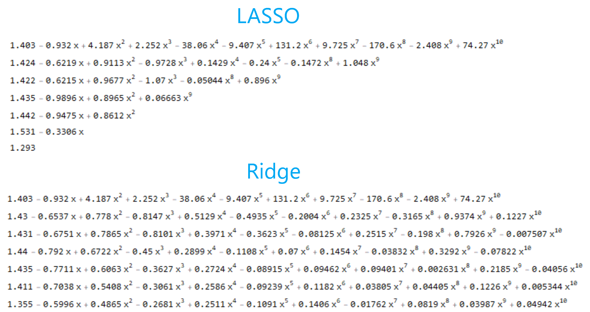
Here is effect of \(\lambda\)’s value on a regression model with 11 variables and LASSO regularization.

Same idea but ridge regularization instead.

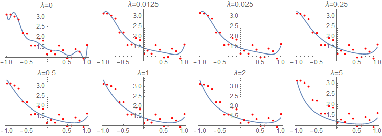
And here you can see how LASSO regularization invokes sparsity by driving some of the model’s parameters to become zero, with increasing values of \(\lambda\). On the contrary, ridge regression keeps every parameter of the model small without forcing it to become zero.

Feature selection

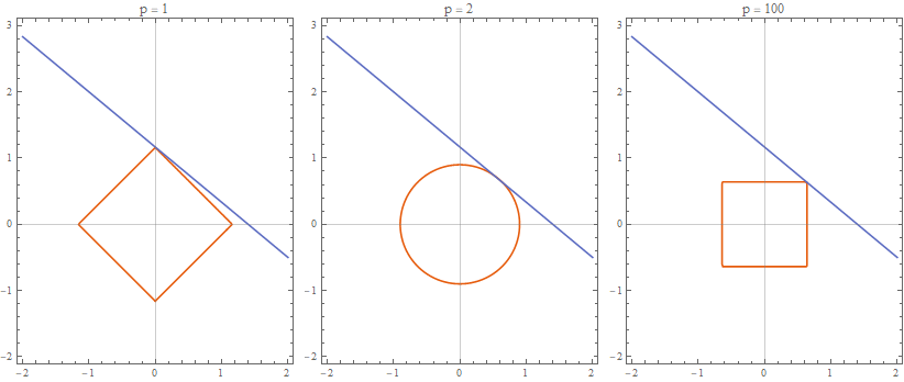
Suppose that we would like to minimize \({\lVert x \rVert}_p\) subject to the constraint \(5x + 6y = 7\), for various values of \(p\). We would start from the center of the axes and we would “blow up” our norm until its boundary intersected with the line \(5x + 6y = 7\). As you can see from the following pictures, for different norms, the optimal point (i.e. the point of the intersection) in \(\mathbb{R}^2\) is different.

And here are the same graphs superimposed.

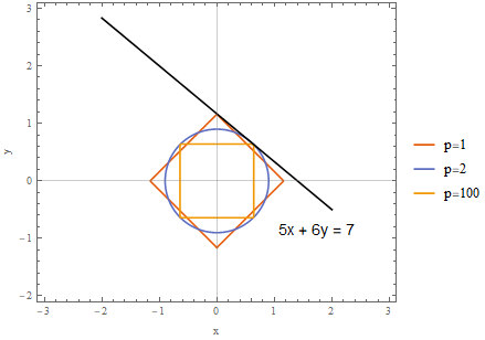
In \(\ell_1\) regularization, our optimization constraint (the line \(5x + 6y = 7\)) intersects with our optimization objective (minimization of the \(\lVert w \rVert_1\) norm) on the \(y\) axis. Therefore, the model’s parameter \(x\) is “forced” to become zero, since the intersection point lies on the \(y\) axis. This is not the case for \(\ell_2\) where the constraint meets the objective outside the \(x\) and \(y\) axes.

Convexity of the norms

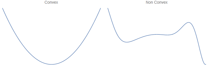
The notion of convexity is the subject of an entire subfield of mathematics. A function \(f\) is called convex if \(\forall x_1, x_2 \in \mathrm{dom}(f), \forall \alpha \in [0, 1]\):

\[f(\alpha x_1+(1-\alpha)x_2)\leq \alpha f(x_1)+(1-\alpha)f(x_2)\]

Mind that the domain of \(f\) must also be a convex set. Here is an example of a convex versus a non-convex function.

Such functions have this nice property, optimization-wise, that any local minimum is also a global minimum. In other words, the function always dominates its first order (linear) Taylor approximation:

\[f(x) \ge f(x_0) + \nabla f(x)^T (x - x_0)\]

Convex functions play nicely with gradient descent. Now, the very definition of a norm implies that a norm is always a convex function. Let \(f = \lVert \cdot \rVert\), then:

\[\underbrace{\|\alpha v+(1-\alpha)w\| \le \|\alpha v\|+\|(1-\alpha)w\|}_\text{triangle inequality} = \underbrace{\alpha\|v\|+(1- \alpha)\|w\|}_\text{scalability}\]

So, by using a cost function that happens to be the norm of a vector space, we end up with a convex optimization function that behaves very well. Also, adding a penalty term from, say, \(\ell_p\) norm preserves the convexity of the cost function (assuming it was convex before, obviously). Because the sum of two convex functions is also a convex function.