Probabilistic regression with Tensorflow
algorithms machine learning Python TensorflowContents
Introduction
You probably have heard the saying, “If all you have is a hammer, everything looks like a nail”. This proverb applies to many cases, deterministic classification neural networks not being an exception. Consider, for instance, a typical neural network that classifies images from the CIFAR-10 dataset. This dataset consists of 60.000 color images, all of which belong to 10 classes: airplanes, cars, birds, cats, deer, dogs, frogs, horses, ships, and trucks. Naturally, no matter what image we feed this network, say a pencil, it will always assign it to one of the 10 known classes.
However, it would be handy if the model conveyed its uncertainty for the predictions it made. So, given a “pencil” image, it would probably label it as a bird or ship or whatever. At the same time, we’d like it to assign a large uncertainty to this prediction. To reach such an inference level, we need to rethink the traditional deterministic neural network paradigm and take a leap of faith towards probabilistic modeling. Instead of having a model parameterized by its point weights, each weight will now be sampled from a posterior distribution whose parameters will be tuned during the training process.
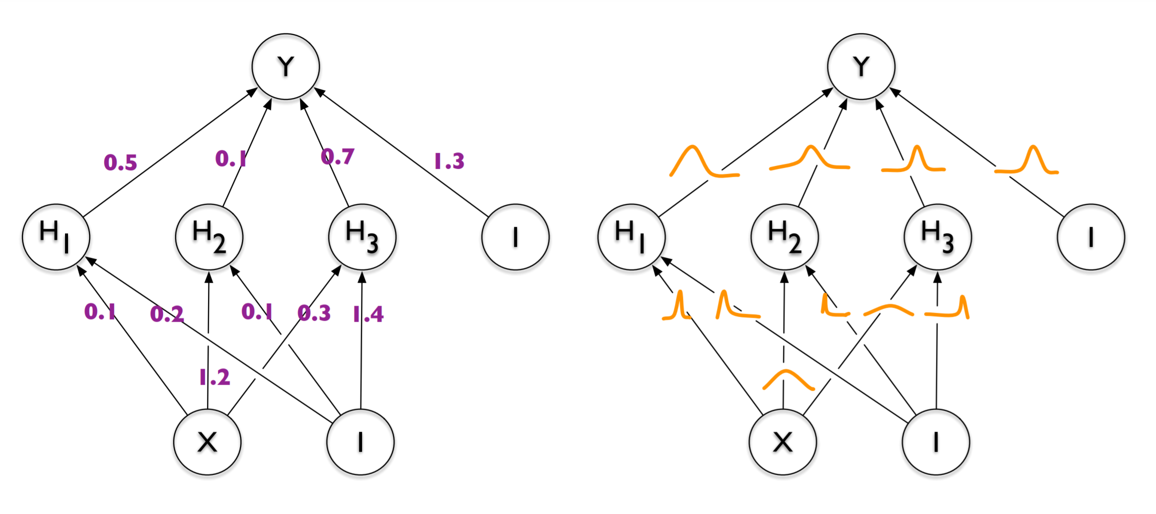
Left: Deterministic neural network with point estimates for weights. Right: Probabilistic neural network with weights sampled from probability distributions. Image taken from Blundell, et al. Weight Uncertainty in Neural Networks. arXiv (2015)
Aleatoric and epistemic uncertainty
Probabilistic modeling is intimately related to the concept of uncertainty. The latter is sometimes divided into two categories, aleatoric (also known as statistical) and epistemic (also known as systematic). Aleatoric is derived from the Latin word “alea” which means die. You might be familiar with the phrase “alea iact est”, meaning “the die has been cast”. Hence, aleatoric uncertainty relates to the data itself and captures the inherent randomness when running the same experiment or performing the same task. For instance, if a person draws the number “4” repeatedly, its shape will be slightly different every time. Aleatoric uncertainty is irreducible in the sense that no matter how much data we collect, there will always be some noise in them. Finally, we model aleatoric uncertainty by having our model’s output be a distribution, where we sample from, rather than having point estimates as output values.
Epistemic uncertainty, on the other hand, refers to a model’s uncertainty. I.e., the uncertainty regarding which parameters (out of the set of all possible parameters) accurately model the experimental data. Epistemic uncertainty is decreased as we collect more training examples. Its modeling is realized by enabling a neural network’s weights to be probabilistic rather than deterministic.
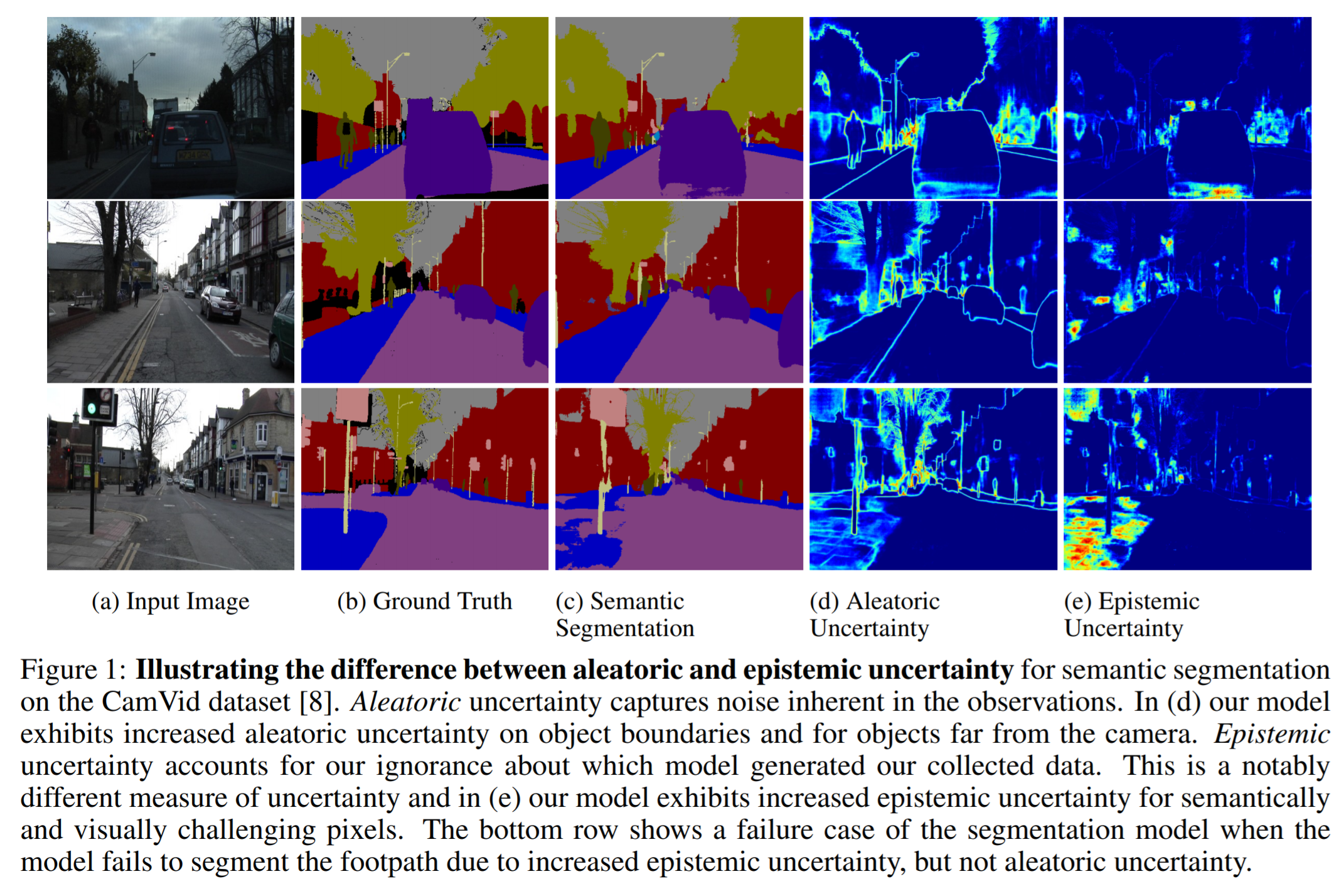
Image taken from Kendall, A. & Gal, Y. What Uncertainties Do We Need in Bayesian Deep Learning for Computer Vision? arXiv [cs.CV] (2017)
Tensorflow example
Summary objective
In the following example, we will generate some non-linear noisy training data, and then we will develop a probabilistic regression neural network to fit the data. To do so, we will provide appropriate prior and posterior trainable probability distributions. This blog post is inspired by a weekly assignment of the course “Probabilistic Deep Learning with TensorFlow 2” from Imperial College London. We start by importing the Python modules that we will need.
import tensorflow as tf
import tensorflow_probability as tfp
tfd = tfp.distributions
tfpl = tfp.layers

import numpy as np
import matplotlib.pyplot as plt
import seaborn as sns
Data generation
We generate some training data \(\mathcal{D}=\{(x_i, y_i)\}\) using the quintic equation \(y_i = x_i^5 + 0.4 \, x_i \,\epsilon_i\) where \(\epsilon_i \sim \mathcal{N}(0,1)\) means that the noise \(\epsilon_i\) is sampled from a normal distribution with zero mean and standard deviation equal to one.
# Generate some non-linear noisy training data
n_points = 500
x_train = np.linspace(-1, 1, n_points)[:, np.newaxis]
y_train = np.power(x_train, 5) + 0.4 * x_train * np.random.randn(n_points)[:, np.newaxis]
plt.scatter(x_train, y_train, alpha=0.2);
plt.xlabel('x')
plt.ylabel('y')
plt.show();
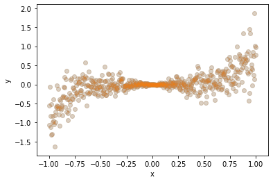
Notice how the data points are squeezed near \(x=0\), and how they diverge as \(x\) deviates from zero. When aleatoric uncertainty (read: measurement noise) differs across the input points \(x\), we call it heteroscedastic, from the Greek words “hetero” (different) and “scedastic” (dispersive). When it is the same for all input, we call it “homoscedastic”.
Setup prior and posterior distributions
Bayes’ rule
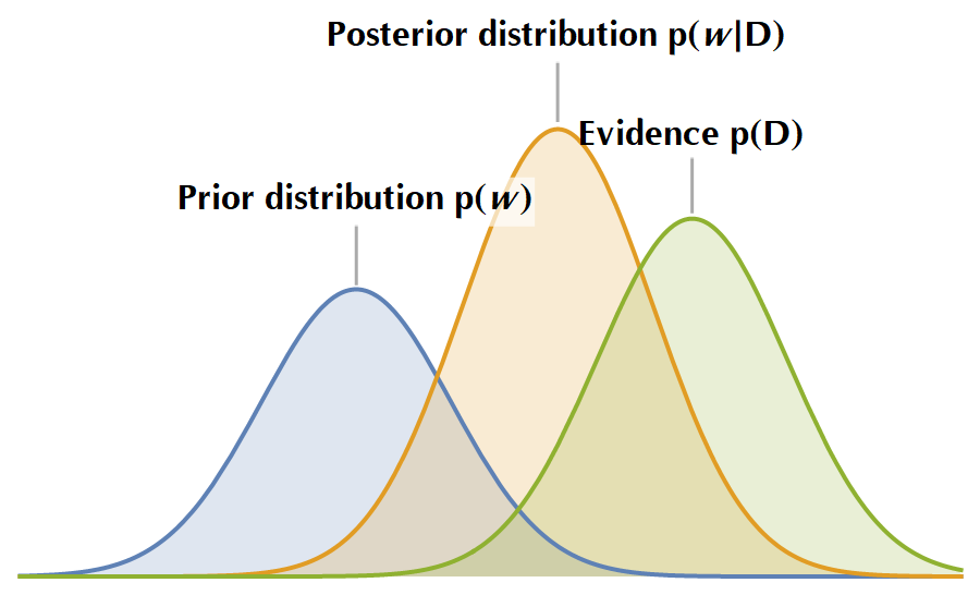
At the core of probabilistic predictive modeling lies the Bayes’ rule. To estimate a full posterior distribution of the parameters \(\mathbf{w}\), i.e., to estimate \(p(\mathbf{w}\mid \mathcal{D})\), given some training data \(\mathcal{D} = \{(x_i, y_i)\}\), the Bayes’ rule assumes the following form:
\[P(\mathbf{\mathbf{w}|\mathcal{D}}) = \frac{P(\mathcal{D}|\mathbf{w})P(\mathbf{w})}{P(\mathcal{D})}\]In the following image, you see a sketch of the various probability distributions that the Bayes’ rule entangles. In plain terms, it holds that \(\text{Prior beliefs} \oplus \text{Evidence} = \text{Posterior beliefs}\), i.e., we start with some assumptions inscribed in the prior distribution, then we observe the “Evidence”, and we update our prior beliefs accordingly, to yield the posterior distribution. Subsequently, the posterior distribution acts as the next iteration’s prior distribution, and the whole cycle is repeated.
To let all these sink, let us elaborate on the essence of the posterior distribution by marginalizing the model’s parameters. The probability of predicting \(y\) given an input \(\mathbf{x}\) and the training data \(\mathcal{D}\) is:
\[P(y\mid \mathbf{x},\mathcal{D})= \int P(y\mid \mathbf{x},\mathbf{w}) \, P(\mathbf{w}\mid\mathcal{D}) \mathop{\mathrm{d}\mathbf{w}}\]This is equivalent to having an ensemble of models with different parameters \(\mathbf{w}\), and taking their average weighted by the posterior probabilities of their parameters, \(P(\mathbf{w}\mid \mathcal{D})\). Neat?
There are two problems with this approach, however. First, it is computationally intractable to calculate an exact solution for the posterior distribution. Second, the averaging implies that our equation is not differentiable, so we can’t use good old backpropagation to update the model’s parameters! The answer to these hindrances is variational inference, a method of formulating inference as an optimization problem. We won’t dive deep into the theoretical background, but the inquiring reader may google for the Kullback-Leibler divergence. The basic idea is to approximate the true posterior with another function by using the KL divergence as a “metric” of how much the two distributions differ. I promise to blog about all the juicy mathematical details of the KL divergence concept in a future post.
Prior distribution
We start by defining a prior distribution for our model’s weights. I haven’t researched the matter a lot, but in the absence of any evidence, adopting a normal distribution as a prior is a fair way to initialize a probabilistic neural network. After all, the central limit theorem asserts that a properly normalized sum of samples will approximate a normal distribution no matter the actual underlying distribution. We use the DistributionLambda() function to inject a distribution into our model, which you can think of as the “lambda function” analog for distributions. The distribution we use is a multivariate normal with a diagonal covariance matrix:
The mean values are initialized to zero and the \(\sigma_i^2\) to one.
def get_prior(kernel_size, bias_size, dtype=None):
    n = kernel_size + bias_size
    prior_model = tf.keras.Sequential([
        tfpl.DistributionLambda(lambda t: tfd.MultivariateNormalDiag(
        loc=tf.zeros(n), scale_diag=tf.ones(n)))
    ])
    return prior_model
Posterior distribution
The case of the posterior distribution is a bit more complex. We again use a multivariate Gaussian distribution, but we will now allow off-diagonal elements in the covariance matrix to be non-zero. There are three ways to parameterize such a distribution. First, in terms of a positive definite covariance matrix \(\mathbf{\Sigma}\), second via a positive definite precision matrix \(\mathbf{\Sigma}^{-1}\), and last with a lower-triangular matrix \(\mathbf{L}\mathbf{L}^⊤\) with positive-valued diagonal entries, such that \(\mathbf{\Sigma} = \mathbf{L}\mathbf{L}^⊤\). This triangular matrix can be obtained via, e.g., Cholesky decomposition of the covariance matrix. In our case, we are going for the last method with MultivariateNormalTriL(), where “TriL” stands for “triangular lower”.
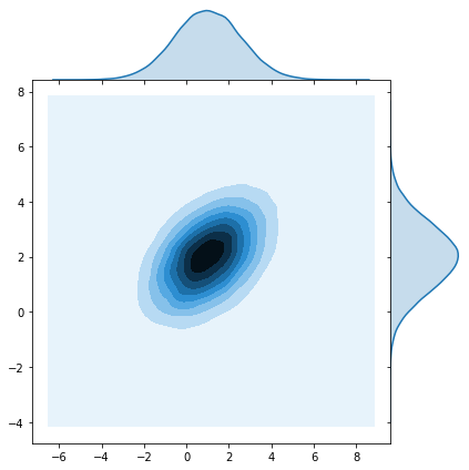
The following parenthetical code shows how one can sample from a multinormal distribution, by setting \(\mathbf{z} = \mathbf{\mu} + \mathbf{L} \mathbf{x}\), where \(\mathbf{\mu}\) is the mean vector, and \(\mathbf{L}\) is the lower triangular matrix derived via \(\mathbf{\Sigma} = \mathbf{L} \mathbf{L}^⊤\) decomposition. The rationale is that sampling from a univariate normal distribution (e.g., zero mean and unit variance) is easy and fast since efficient vectorized algorithms exist for doing this. Whereas sampling directly from a multinormal distribution is not as efficient. Hence, we turn the problem of sampling a multinormal distribution into sampling a univariate normal.
# Define the mean vector mu
mu = np.array([1, 2]).reshape(2, 1)

# Define the covariance matrix (it must be positive definite)
K = np.array([[2, 1],
              [1, 2]])

# Apply Cholesky decomposition of K to LL^T
L = np.linalg.cholesky(K)
L = L.T

# The variable z follows a multinormal distribution
n_samples = 100000
x = np.random.normal(loc=0, scale=1, size=2*n_samples).reshape(2, n_samples)
z = mu + np.dot(L, x)

sns.jointplot(x=z[0], y=z[1], kind="kde");
So, instead of parameterizing the neural network with point estimates for weights \(\mathbf{w}\), we will instead parameterize it with \(\mathbf{\mu}\)’s and \(\sigma\)’s. Notice that for a lower triangular matrix there are \((n^2 - n)/2 + n = n(n+1)/2\) non-zero elements. Adding the \(n\) \(\mu\)’s we end up with a distribution with \(n(n+1)/2 + n = n(n+3)/2\) parameters.
def get_posterior(kernel_size, bias_size, dtype=None):
    n = kernel_size + bias_size
    posterior_model = tf.keras.Sequential([
        tfpl.VariableLayer(tfpl.MultivariateNormalTriL.params_size(n), dtype=dtype),
        tfpl.MultivariateNormalTriL(n)
    ])
    return posterior_model
By the way, let us create some prior and posterior distributions, print the number of their trainable variables, and sample from them. Note that every time we run this cell block, we get different results for the samples.
# The prior distribution has no trainable variables
prior_model = get_prior(3, 1)
print('Trainable variables for prior model: ', prior_model.layers[0].trainable_variables)
print('Sampling from the prior distribution:\n', prior_model.call(tf.constant(1.0)).sample(5))

# The posterior distribution for kernel_size = 3, bias_size = 1, is expected to
# have (3 + 1) + ((4^2 - 4)/2 + 4) = 14 parameters. Note that the default initializer
# according to the docs is 'zeros'.
posterior_model = get_posterior(3, 1)
print('\nTrainable variables for posterior model: ', posterior_model.layers[0].trainable_variables)
print('Sampling from the posterior distribution:\n', posterior_model.call(tf.constant(1.0)).sample(5))

#    Trainable variables for prior model:  []
#    Sampling from the prior distribution:
#     tf.Tensor(
#    [[ 1.3140054   0.93301576 -2.3522265   0.5879774 ]
#     [-2.6143072   0.39889303  0.72736305 -0.06531376]
#     [-1.1271048   0.4480154  -1.389969    0.87443566]
#     [-0.6140247   0.3008949   0.91000426  0.1832995 ]
#     [ 0.39756483  0.4414646  -1.025012    0.21117625]], shape=(5, 4), dtype=float32)
#
#    Trainable variables for posterior model:  [<tf.Variable 'constant:0' shape=(14,) dtype=float32, numpy=
#    array([0., 0., 0., 0., 0., 0., 0., 0., 0., 0., 0., 0., 0., 0.],
#          dtype=float32)>]
#    Sampling from the posterior distribution:
#     tf.Tensor(
#    [[-0.0099524   1.107596   -0.34787297  0.1307174 ]
#     [-0.7565929  -0.08078367  0.1275031   0.80345786]
#     [ 0.75810474  0.12409975  0.11558666  0.54518634]
#     [-0.5074226   0.11740679  0.86849195 -0.33246624]
#     [ 0.01261052  0.44296038  0.61944205  0.4496125 ]], shape=(5, 4), dtype=float32)
Define the model, loss function, and optimizer
To define probabilistic layers in a neural network, we use the DenseVariational() function, specifying the input and output shape, along with the prior and posterior distributions that we have previously defined. We use a sigmoid activation function to enable the network model non-linear data, along with an IndependentNormal() output layer, to capture aleatoric uncertainty, with an event shape equal to 1 (since our \(y\) is just a scalar). Regarding the kl_weight parameter, you may refer to the original paper “Weight Uncertainty in Neural Networks” for further information. For now, just take for granted that it is a scaling factor.
# Define the model, negative-log likelihood as the loss function
# and compile the model with the RMSprop optimizer
model = tf.keras.Sequential([
    tfpl.DenseVariational(input_shape=(1,), units=8,
                          make_prior_fn=get_prior,
                          make_posterior_fn=get_posterior,
                          kl_weight=1/x_train.shape[0],
                          activation='sigmoid'),
    tfpl.DenseVariational(units=tfpl.IndependentNormal.params_size(1),
                          make_prior_fn=get_prior,
                          make_posterior_fn=get_posterior,
                          kl_weight=1/x_train.shape[0]),
    tfpl.IndependentNormal(1)
])

def nll(y_true, y_pred):
    return -y_pred.log_prob(y_true)

model.compile(loss=nll, optimizer=tf.keras.optimizers.RMSprop(learning_rate=0.005))
model.summary()

#    Model: "sequential_2"
#    _________________________________________________________________
#    Layer (type)                 Output Shape              Param #
#    =================================================================
#    dense_variational (DenseVari (None, 8)                 152
#    _________________________________________________________________
#    dense_variational_1 (DenseVa (None, 2)                 189
#    _________________________________________________________________
#    independent_normal (Independ multiple                  0
#    =================================================================
#    Total params: 341
#    Trainable params: 341
#    Non-trainable params: 0
#    _________________________________________________________________
Let’s practice and calculate by hand the model’s parameters. The first dense variational layer has 1 input, 8 outputs and 8 biases. Therefore, there are \(1\cdot 8 + 8 = 16\) weights. Since each weight is going to be modelled by a normal distribution, we need 16 \(\mu\)’s, and \((16^2 - 16)/2 + 16 = 136\) \(\sigma\)’s. The latter is just the number of elements of a lower triangular matrix \(16\times 16\). Therefore, in total we need \(16 + 136 = 152\) parameters.
What about the second variational layer? This one has 8 inputs (since the previous had 8 outputs), 2 outputs (the \(\mu, \sigma\) of the independent normal distribution), and 2 biases. Therefore, it has \(8\times 2 + 2 = 18\) weights. For 18 weights, we need 18 \(\mu\)’s and \((18^2 - 18)/2 + 18 = 171\) \(\sigma\)’s. Therefore, in total we need \(18 + 171 = 189\) parameters. The tfpl.MultivariateNormalTriL.params_size(n) static function calculates the number of parameters needed to parameterize a multivariate normal distribution, so that we don’t have to bother with it.
Train the model and make predictions
We train the model for 1000 epochs and plot the loss function vs. to confirm that the algorithm has converged.
# Train the model for 1000 epochs
history = model.fit(x_train, y_train, epochs=1000, verbose=0)
plt.plot(history.history['loss'])
plt.xlabel('Epochs')
plt.ylabel('Loss');
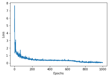
Indeed RMSprop converged, and now we proceed by making some predictions:
plt.scatter(x_train, y_train, marker='.', alpha=0.2, label='data')
for _ in range(5):
    y_model = model(x_train)
    y_hat = y_model.mean()
    y_hat_minus_2sd = y_hat - 2 * y_model.stddev()
    y_hat_plus_2sd = y_hat + 2 * y_model.stddev()
    plt.plot(x_train, y_hat, color='red', label='model $\mu$' if _ == 0 else '')
    plt.plot(x_train, y_hat_minus_2sd, color='blue', label='$\mu - 2SD$' if _ == 0 else '')
    plt.plot(x_train, y_hat_plus_2sd, color='green', label='$\mu + 2SD$' if _ == 0 else '')
plt.xlabel('x')
plt.ylabel('y')
plt.legend()
plt.show()
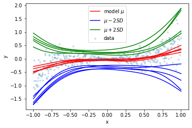
Notice how the models’ outputs converge around \(x=0\) where there is very little variation in the data. The following plot was generated by taking the average of 100 models:
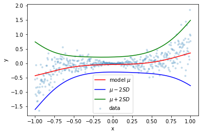
In the following two images, you can see how going from known inputs to extrapolating to unknown inputs “forces” our model to spread out its predictions.
| Known input | Unknown input |
|---|---|
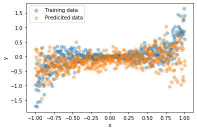 |
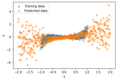 |