The encoder-decoder model as a dimensionality reduction technique
machine learning Principal Component Analysis Python TensorflowContents
- Introduction
- What is an encoder-decoder model?
- A minimal working example
- A more interesting dataset
- Autoencoder vs. Principal Component Analysis
The cool part starts here.
Introduction
In today’s post, we will discuss the encoder-decoder model, or simply autoencoder (AE). This will serve as a basis for implementing the more robust variational autoencoder (VAE) in the following weeks. For starters, we will describe the model briefly and implement a dead simple encoder-decoder model in Tensorflow with Keras, in an absolutely indifferent dataset (my master thesis data). As a reward for enduring my esoteric narrative, we will then proceed to a more exciting dataset, the MNIST, to show how the encoder-decoder model can be used for dimensionality reduction. To spice things up, we will construct a Keras callback to visualize the encoder’s feature representation before each epoch. We will then see how the network builds up its hidden model progressively, epoch by epoch. Finally, we will compare AE to other standard methods, such as principal component analysis. Without further ado, let’s get started!
What is an encoder-decoder model?
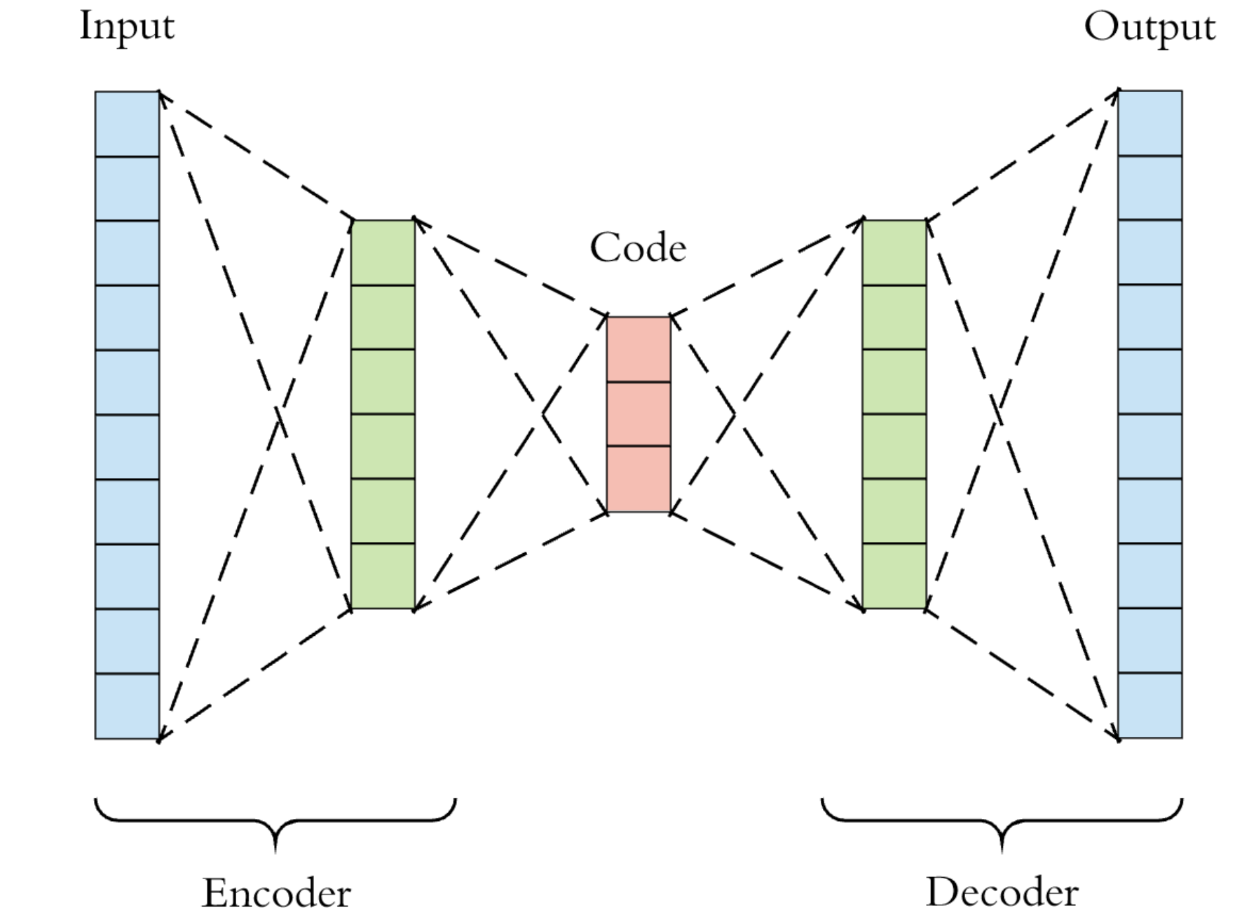
An encoder-decoder network is an unsupervised artificial neural model that consists of an encoder component and a decoder one (duh!). The encoder takes the input and transforms it into a compressed encoding, handed over to the decoder. The decoder strives to reconstruct the original representation as close as possible. Ultimately, the goal is to learn a representation (read: encoding) for a dataset. In a sense, we force the AE to memorize the training data by devising some mnemonic rule of its own. As you see in the following figure, such a network has, typically, a bottleneck-like shape. It starts wide, then its units/connections are squeezed toward the middle, and then they fan out again. This architecture forces the AE to compress the training data’s informational content, embedding it into a low-dimensional space. By the way, you may encounter the term “latent space” for this data’s intermediate representation space.
A minimal working example
Preprocessing
First, we import the modules and functions we will be using:
import matplotlib.pyplot as plt
import numpy as np
import tensorflow as tf
from tensorflow.keras.models import Model, Sequential
from tensorflow.keras.layers import Dense
import pandas as pd
import random
from sklearn.preprocessing import StandardScaler
The dataset that we will be using is from my master thesis. It consists of 10 complexity indices for volumetric modulated arc therapy plans in prostate cancer. The details don’t really matter; any high-dimensional data would do.
# Load database
pdf = pd.read_excel(r'/home/stathis/Jupyter_Notebooks/datasets/vmat_prostate_complexity.xlsx')
# Select only VMAT plans with radical intent (i.e., skip patients treated postoperatively
# in a salvage or adjuvant setting)
pdf = pdf[pdf['setting'] == 'radical']
# Calculate the combinatorial complexity index LTMCSV = LT * MCSV
pdf['ltmcsv'] = pdf['lt'] * pdf['mcsv']
# Select only the columns corresponding to the desired complexity metrics
metric_names = ['coa', 'em', 'esf', 'lt', 'ltmcsv', 'mcs', 'mcsv', 'mfa', 'pi', 'sas']
npdf = pdf[metric_names]
# Convert pandas dataframe to numpy array
x_train = npdf.to_numpy()
# Scale data to have zero mean and unit variance
scaler = StandardScaler()
scaler.fit(x_train)
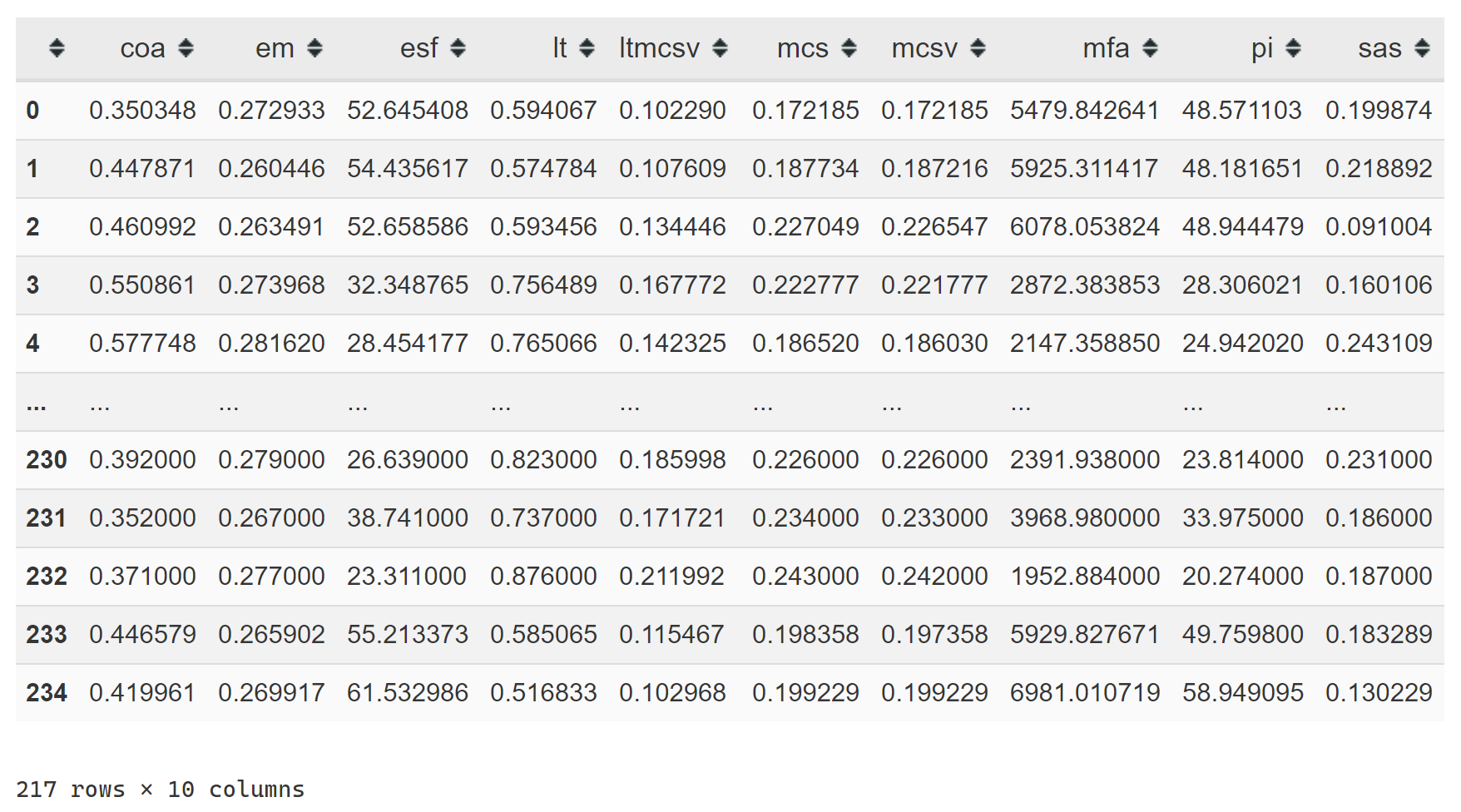
x_train = scaler.transform(x_train)The data look like this:
Building the autoencoder
Next, we build our autoencoder’s architecture. We will squeeze the 10-dimensional space into a 2-dimensional latent space. Our choices regarding the model’s architecture are very rudimentary; the goal is to demonstrate how an encoder works, not design the optimal one.
# This is the dimension of the original space
input_dim = 10

# This is the dimension of the latent space (encoding space)
latent_dim = 2

encoder = Sequential([
    Dense(128, activation='relu', input_shape=(input_dim,)),
    Dense(64, activation='relu'),
    Dense(32, activation='relu'),
    Dense(latent_dim, activation='relu')
])

decoder = Sequential([
    Dense(64, activation='relu', input_shape=(latent_dim,)),
    Dense(128, activation='relu'),
    Dense(256, activation='relu'),
    Dense(input_dim, activation=None)
])
Here comes the “surgical” part of the work. We stitch up the encoder and the decoder models into a single model, the autoencoder. The autoencoder’s input is the encoder’s input, and the autoencoder’s output is the decoder’s output. The output of the decoder is the result of calling the decoder on the output of the encoder. We also set the loss to mean squared error.
autoencoder = Model(inputs=encoder.input, outputs=decoder(encoder.output))
autoencoder.compile(loss='mse', optimizer='adam')
At this point, our autoencoder has not been trained yet. Let’s feed it with some examples from the dataset and see how well it performs in reconstructing the input.
def plot_orig_vs_recon(title='', n_samples=3):
    fig = plt.figure(figsize=(10,6))
    plt.suptitle(title)
    for i in range(3):
        plt.subplot(3, 1, i+1)
        idx = random.sample(range(x_train.shape[0]), 1)
        plt.plot(autoencoder.predict(x_train[idx]).squeeze(), label='reconstructed' if i == 0 else '')
        plt.plot(x_train[idx].squeeze(), label='original' if i == 0 else '')
        fig.axes[i].set_xticklabels(metric_names)
        plt.xticks(np.arange(0, 10, 1))
        plt.grid(True)
        if i == 0: plt.legend();

plot_orig_vs_recon('Before training the encoder-decoder')
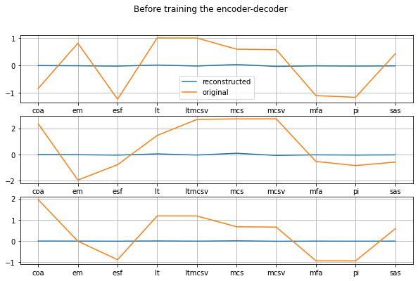
Great! The autoencoder does not work at all! It would be very spooky to see it replicate the input without having been trained to do so ;)
Training the autoencoder
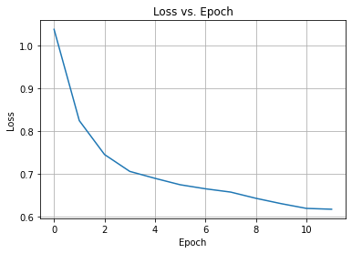
We then train the model for 5000 epochs and check the loss vs. epoch to make sure that it converged. Notice how the input and the output training data are the same, the x_train.
model_history = autoencoder.fit(x_train, x_train, epochs=5000, batch_size=32, verbose=0)

plt.plot(model_history.history["loss"])
plt.title("Loss vs. Epoch")
plt.ylabel("Loss")
plt.xlabel("Epoch")
plt.grid(True)
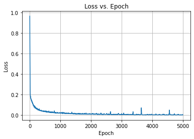
Woot. The optimizer converged, so we can check again how well the autoencoder can reconstruct its input.
plot_orig_vs_recon('After training the encoder-decoder')
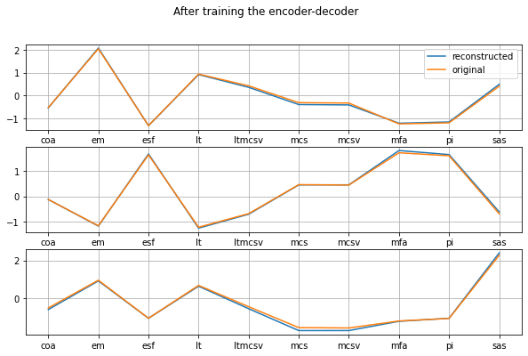
That’s pretty damn good. The reconstructed values are very close to the original ones! Now let’s take a look at the latent space. Since we set it to be 2-dimensional, we will use a 2D scatterplot to visualize it. This is the projection of the 10-dimensional data onto a plane.
encoded_x_train = encoder(x_train)
plt.figure(figsize=(6,6))
plt.scatter(encoded_x_train[:, 0], encoded_x_train[:, 1], alpha=.8)
plt.xlabel('Latent Dimension 1')
plt.ylabel('Latent Dimension 2');
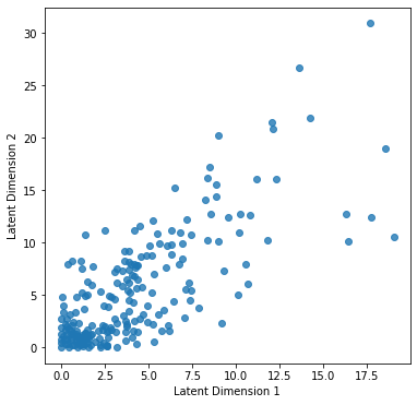
This 2D imprint is all it takes for the decoder to regenerate the initial 10-dimensional space. Isn’t it awesome? Notice, though, that there are lots of points crowded in the bottom left corner. Ideally, we would like each class’s data points to form distinct clusters in a classification scenario. E.g., if our data were furniture, we would like chairs to be projected at the bottom left corner, tables to the bottom right, and so on. In the next example, we will make this happen, and as a matter of fact, we will watch it happening live during the training process.
A more interesting dataset
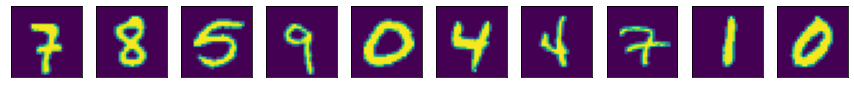
We now move forward to the MNIST dataset. This consists of a training set of 60.000 examples and a test set of 10.000 samples. Each example is a 28x28 grayscale image of a handwritten digit from 0 to 9. When I wrote this blog post, I thought that I had been using the Fashion MNIST dataset. The latter has been proposed as a replacement for the original MNIST dataset when benchmarking machine learning algorithms. I then realized that I had loaded the regular MNIST dataset but was too lazy to regenerate the plots for the Fashion MNIST. Hence, this is left as an exercise to the reader! :D
Preprocessing
# Load the MNIST data set
(x_train, y_train), (x_test, y_test) = tf.keras.datasets.mnist.load_data()

# Normalize pixel values to [0., 1.]
x_train = x_train / 255.
x_test = x_test / 255.

# Take a look at the dataset
n_samples = 10
idx = random.sample(range(x_train.shape[0]), n_samples)
plt.figure(figsize=(15,4))
for i in range(n_samples):
    plt.subplot(1, n_samples, i+1)
    plt.imshow(x_train[idx[i]].squeeze());
    plt.xticks([], [])
    plt.yticks([], [])
Building the autoencoder
The same as before, we set up the autoencoder. Please keep in mind that whatever has to do with image classification works better with convolutional neural networks of some sort. However, here we keep it simple and go with dense layers. Feel free to change the number of layers, the number of units, and the activation functions. My choice is by no way optimal nor the result of an exhaustive exploration.
# This is the dimension of the latent space (encoding space)
latent_dim = 2

# Images are 28 by 28
img_shape = (x_train.shape[1], x_train.shape[2])

encoder = Sequential([
    Flatten(input_shape=img_shape),
    Dense(192, activation='sigmoid'),
    Dense(64, activation='sigmoid'),
    Dense(32, activation='sigmoid'),
    Dense(latent_dim, name='encoder_output')
])

decoder = Sequential([
    Dense(64, activation='sigmoid', input_shape=(latent_dim,)),
    Dense(128, activation='sigmoid'),
    Dense(img_shape[0] * img_shape[1], activation='relu'),
    Reshape(img_shape)
])
Creating a custom callback
Here comes the cool part. To visualize how the autoencoder builds up the latent space representation, as we train it, we will create a custom callback by subclassing the tf.keras.callbacks.Callback. We will then override the method on_epoch_begin(self, epoch, logs=None), which is called at the beginning of an epoch during training. There, we will hook up our code to extract the latent space representation and plot it. To obtain the output of an intermediate layer (in our case, we want to extract the encoder’s output), we will retrieve it via the layer.output. Here’s how:
class TestEncoder(tf.keras.callbacks.Callback):
    def __init__(self, x_test, y_test):
        super(TestEncoder, self).__init__()
        self.x_test = x_test
        self.y_test = y_test
        self.current_epoch = 0

    def on_epoch_begin(self, epoch, logs={}):
        self.current_epoch = self.current_epoch + 1
        encoder_model = Model(inputs=self.model.input,
                              outputs=self.model.get_layer('encoder_output').output)
        encoder_output = encoder_model(self.x_test)
        plt.subplot(4, 3, self.current_epoch)
        plt.scatter(encoder_output[:, 0],
                    encoder_output[:, 1], s=20, alpha=0.8,
                    cmap='Set1', c=self.y_test[0:x_test.shape[0]])
        plt.xlim(-9, 9)
        plt.ylim(-9, 9)
        plt.xlabel('Latent Dimension 1')
        plt.ylabel('Latent Dimension 2')

autoencoder = Model(inputs=encoder.input, outputs=decoder(encoder.output))
autoencoder.compile(loss='binary_crossentropy', optimizer='adam')
Training the autoencoder
Off to train the model!
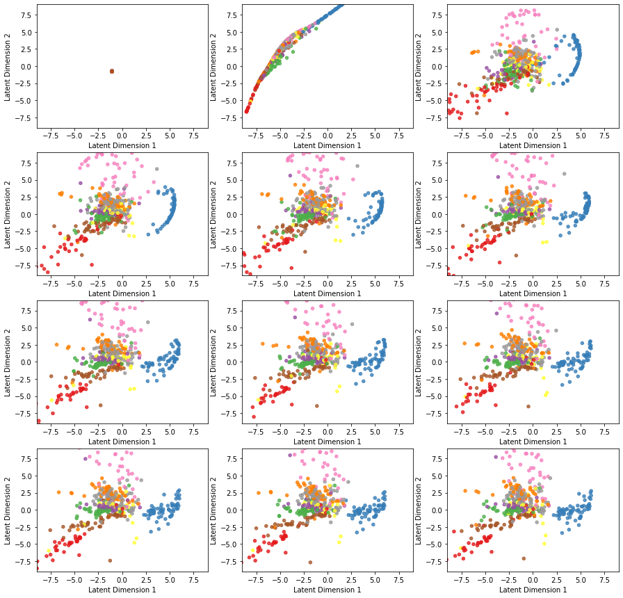
plt.figure(figsize=(15,15))
model_history = autoencoder.fit(x_train, x_train, epochs=12, batch_size=32, verbose=0,
                                callbacks=[TestEncoder(x_test[0:500], y_test[0:500])])
Here is the evolution of latent space representation as the autoencoder is trained, starting with an untrained state at the top left and ending in a fully trained state at the bottom right. Before the first epoch, all the original space data are projected on the same point of the latent space. However, as the autoencoder undergoes training, the points corresponding to different classes start to separate.
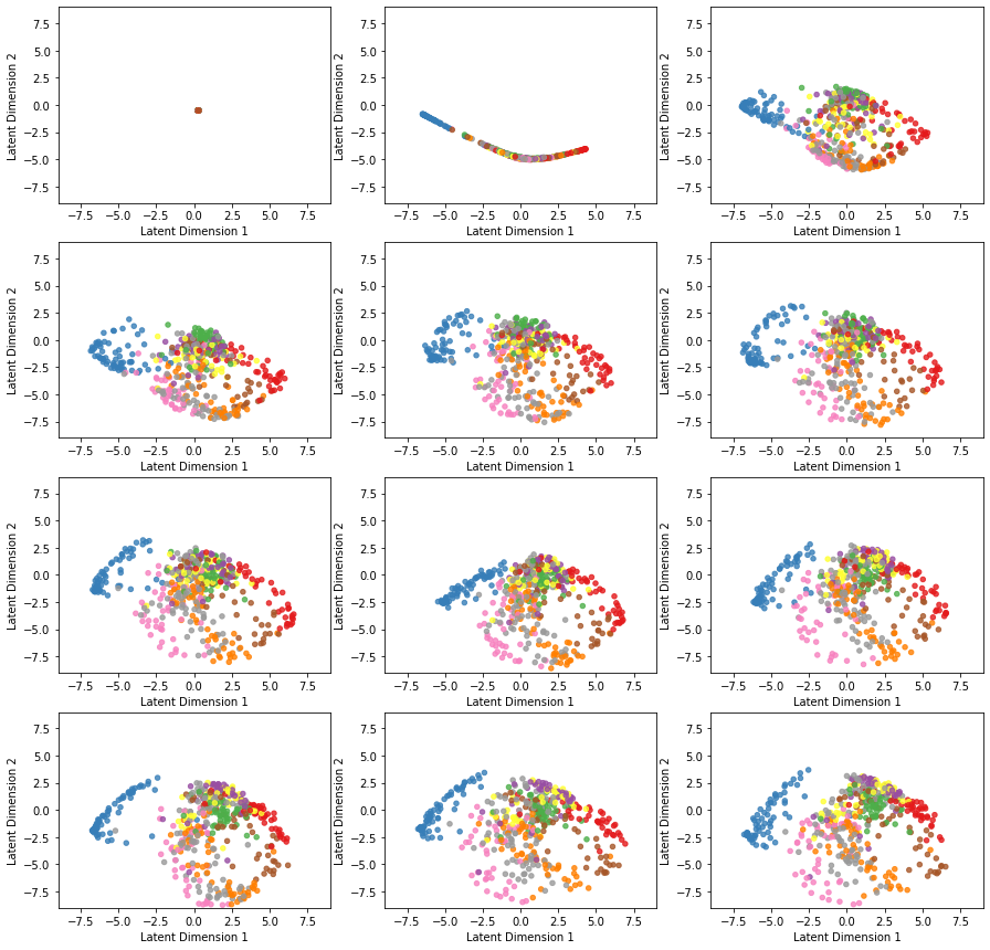
We check the loss vs. epoch to make sure the optimizer converged. We may even observe a correspondence between the classes’ separation and how fast the loss is minimized during the training.
plt.plot(model_history.history["loss"])
plt.title("Loss vs. Epoch")
plt.ylabel("Loss")
plt.xlabel("Epoch")
plt.grid(True)
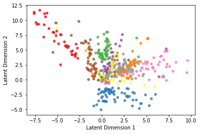
We now change the activation function of the last dense layer in the decoder from relu to sigmoid, and we retrain the model. Notice how the latent representation is different now (actually, it’s better):
This is an animation that I made with an autoencoder model in Mathematica.
Latent space vs. Principal components space
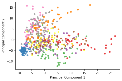
Finally, let’s look at the PCA decomposition of the MNIST dataset assuming 2 principal components.
pca = PCA(n_components=2)
x_reshaped = x_test[0:500].reshape(-1, 784)              # new shape is (500, 28*28) = (500, 784)
x_scaled = StandardScaler().fit_transform(x_reshaped)    # center and scale data (mean=0, std=1)
x_transformed = pca.fit(x_scaled).transform(x_scaled)

plt.figure()
plt.scatter(x_transformed[:, 0], x_transformed[:, 1],
            s=20, alpha=.8, cmap='Set1', c=y_test[0:500])
plt.xlabel('Principal Component 1')
plt.ylabel('Principal Component 2');
And here we plot them side by side:
| Autoencoder latent space representation | PCA decomposition |
|---|---|
 |
|
Autoencoder as a generative model
Once the autoencoder has built a latent representation of the input data set, we could in principle sample a random point of the latent space and use it as input to the decoder to generate a synthetic (fake) image. For example:
n_samples = 40
fake_sample = np.random.uniform(low=-20, high=20, size=(n_samples, 2))
plt.figure(figsize=(15,5))
for i in range(n_samples):
    plt.subplot(4, n_samples//4, i+1)
    fake_encoding = np.array([fake_sample[i]])
    fake_digit = decoder(fake_encoding).numpy().squeeze()
    plt.imshow(fake_digit);
    plt.xticks([], [])
    plt.yticks([], [])
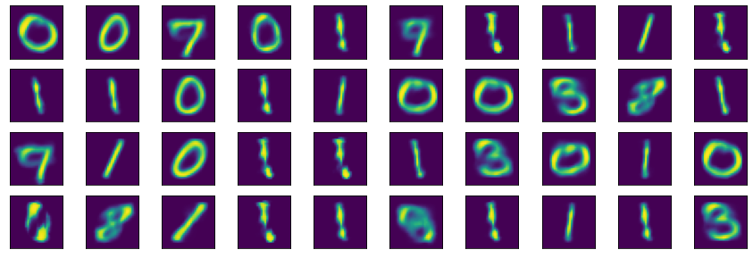
Occasionally, however, the autoencoder will output garbage because our setup does not include any regularization. This lack of regularization leads to severe overfitting. Therefore some points of the latent space will give meaningless content once decoded. After all, we did not ask the autoencoder to organize the latent space representation in some particular way. All we asked was to reconstruct the input without any loss. And the easiest way to accomplish this is to overfit! ;) There are, of course, ways to mitigate overfitting, but that’s for another day!
Autoencoder vs. Principal Component Analysis
As we’ve seen, both autoencoder and PCA may be used as dimensionality reduction techniques. However, there are some differences between the two:
- By definition, PCA is a linear transformation, whereas AEs are capable of modeling complex non-linear functions. There is, however, kernel PCA that can model non-linear data.
- In PCA, features are by definition linearly uncorrelated. Recall that they are projections onto an orthogonal basis. On the contrary, autoencoded features might be correlated. The two optimization objectives are simply different (an orthogonal basis that maximizes variance when data are projected onto it vs. maximum accuracy reconstruction).
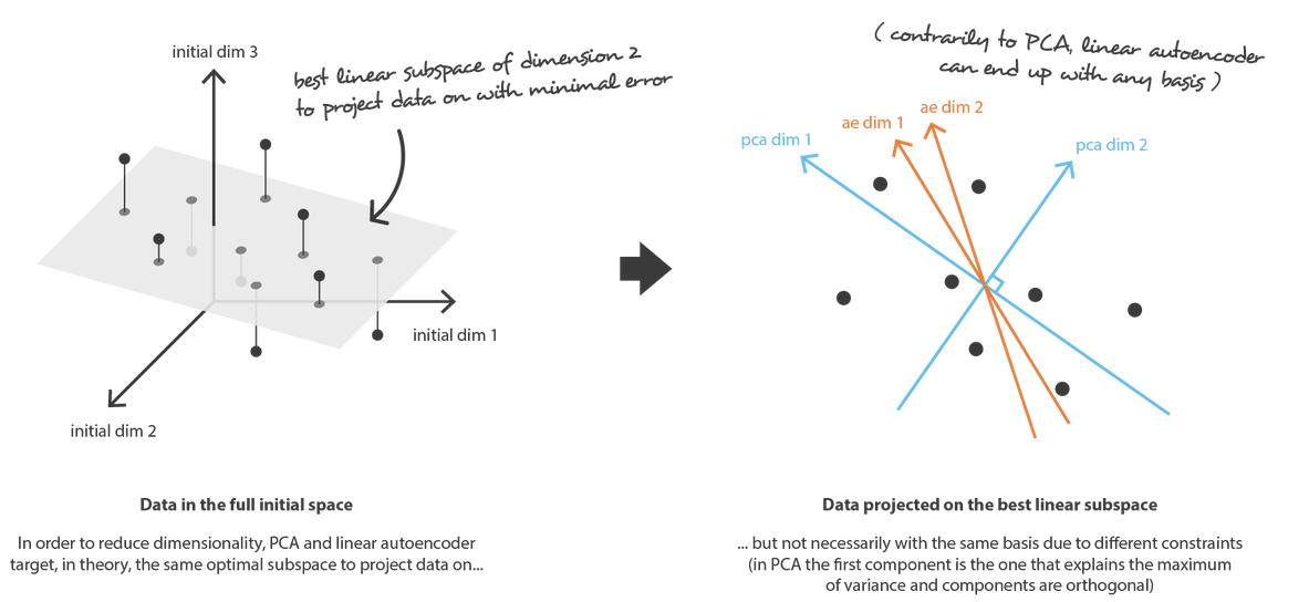
Image taken from here.
- PCA is computationally less demanding than autoencoders. For instance, PCA on the MNIST dataset takes 0.05 seconds +/- 0.008 in my PC, whereas training the AE around 3-4 minutes.
- Autoencoders having many trainable parameters are vulnerable to overfitting, similar to other neural networks.
Regarding the question of which one to use, I’m afraid I’ll sound cliché. It depends on the problem you are trying to solve. If your data share non-linear correlations, AE will compress them into a low-dimensional latent space since it is endowed with the capability to model non-linear functions. If your data are mostly linearly correlated, PCA will do fine. By the way, there’s also a kernel version of PCA. Using a kernel trick, similar to the one with Support Vector Machines, the originally linear operations of PCA are performed in a reproducing kernel space. But that’s the subject of a future post.