Decision Trees: Gini index vs entropy

Introduction

Decision trees are tree-based methods that are used for both regression and classification. They work by segmenting the feature space into several simple subregions. To make predictions, trees assume either the mean or the most frequent class of the training points inside the region our observation falls, depending on whether we do regression or classification, respectively. Decision trees are straightforward to interpret, and as a matter of fact, they can be even easier to interpret than linear or logistic regression models. Perhaps because they relate to how the human decision-making process works. On the downside, trees usually lack the level of predictive accuracy of other methods. Also, they can be susceptible to changes in the training dataset, where a slight change in it may cause a dramatic change in the final tree. That’s why bagging, random forests and boosting are used to construct more robust tree-based prediction models. But that’s for another day. Today we are going to talk about how the split happens.

Gini impurity and information entropy

Trees are constructed via recursive binary splitting of the feature space. In classification scenarios that we will be discussing today, the criteria typically used to decide which feature to split on are the Gini index and information entropy. Both of these measures are pretty similar numerically. They take small values if most observations fall into the same class in a node. Contrastly, they are maximized if there’s an equal number of observations across all classes in a node. A node with mixed classes is called impure, and the Gini index is also known as Gini impurity.

Concretely, for a set of items with \(K\) classes, and \(p_k\) being the fraction of items labeled with class \(k\in {1,2,\ldots,K}\), the Gini impurity is defined as:

\[G = \sum_{k=1}^K p_k (1 - p_k) = 1 - \sum_{k=1}^N p_k^2\]

And information entropy as:

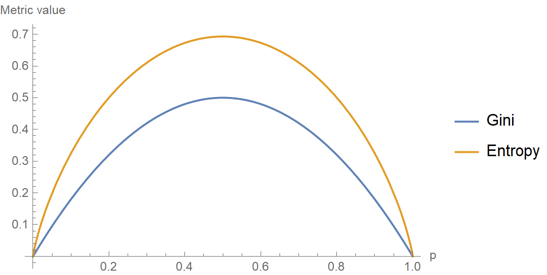
\[H = -\sum_{k=1}^K p_k \log p_k\]

In the following plot, both metrics are plotted against each other, considering a set of K=2 classes with probability \(p\) and \(1-p\), respectively. Notice how for small values of \(p\), Gini is consistently lower than entropy. Therefore, it penalizes less small impurities. This is a crucial observation that will prove helpful in the context of imbalanced datasets.

The Gini index is used by the CART (classification and regression tree) algorithm, whereas information gain via entropy reduction is used by algorithms like C4.5. In the following image, we see a part of a decision tree for predicting whether a person receiving a loan will be able to pay it back. The left node is an example of a low impurity node since most of the observations fall into the same class. Contrast this with the node on the right where observations of different classes are mixed in.

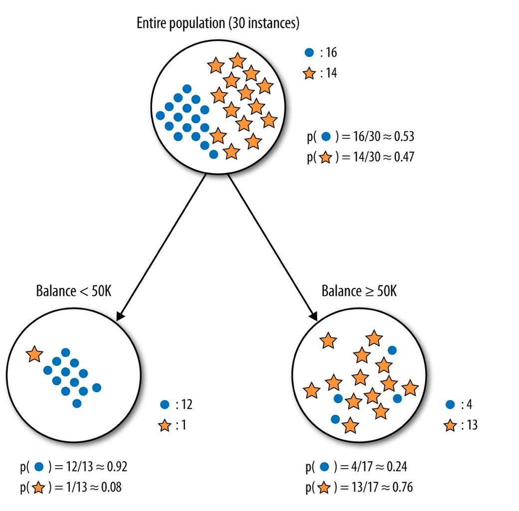
Image taken from “Provost, Foster; Fawcett, Tom. Data Science for Business: What You Need to Know about Data Mining and Data-Analytic Thinking”.

Let’s calculate the Gini impurity of the left node:

\[\begin{align} G\left(\text{Balance < 50K}\right) &= 1-\sum_{k=1}^{2} p_k^2 = 1-p_1^2 - p_2^2\\ &=1-\left(\frac{12}{13}\right)^2 -\left(\frac{1}{13}\right)^2 \simeq 0.14 \end{align}\]

And the Gini impurity of the right node:

\[\begin{align} G\left(\text{Balance} \ge \text{50K}\right) &= 1-\sum_{k=1}^{2} p_k^2 = 1-p_1^2 - p_2^2\\ &=1-\left(\frac{4}{17}\right)^2 -\left(\frac{13}{17}\right)^2 \simeq 0.36 \end{align}\]

We notice that the left node has a lower Gini impurity index, which we’d expect since \(G\) measures impurity, and the left node is purer relative to the right one. Let’s calculate now the entropy of the left node:

\[\begin{align} H\left(\text{Balance < 50K}\right) &= -\sum_{k=1}^{2} p_k \log{p}_k = -p_1 \log{p}_1 -p_2 \log{p}_2\\ &=-\frac{12}{13}\log\left(\frac{12}{13}\right) -\frac{1}{13}\log\left(\frac{1}{13}\right) \simeq 0.27 nats \end{align}\]

Depending on whether we are using \(log_2\) or \(log_e\) in the entropy formula we get the result in bits or nats, respectively. For instance, here it’s \(H \simeq 0.39 bits\). Let’s calculate the entropy of the right node as well:

\[\begin{align} H\left(\text{Balance}\ge\text{50K}\right) &= -\sum_{k=1}^{2} p_k \log{p}_k = -p_1 \log{p}_1 -p_2 \log{p}_2\\ &=-\frac{4}{17}\log\left(\frac{4}{17}\right) -\frac{13}{17}\log\left(\frac{13}{17}\right) \simeq 0.55 nats \end{align}\]

Again, if we’d use base 2 in the entropy’s logarithm, we’d get \(H \simeq 0.79 bits\). Units aside, we see that the left node has lower entropy than the right one, which is expected since the left one is in a more ordered state and entropy measures disorder. So, it’s \(H_\text{left} \simeq 0.27 nats\) and \(H_\text{right} \simeq 0.55 nats\). The various algorithms for assembling decision trees pick the next feature to split, so maximum impurity reduction is achieved.

Let’s calculate how much entropy is reduced by splitting on the “Balance” feature:

\[\begin{align*} H(\text{Parent}) &= -\frac{16}{30} \log\left(\frac{16}{30}\right) -\frac{14}{30}\log\left(\frac{14}{30}\right)\simeq 0.69nats\\ H(\text{Balance}) &= \frac{13}{30} \times 0.27 + \frac{17}{30} \times 0.55 \simeq 0.43nats \end{align*}\]

Therefore, the information gain by splitting on the “Balance” feature is:

\[\text{IG} = H(\text{Parent}) - H(\text{Balance}) = 0.69 - 0.43 = 0.26nats\]

If we were to choose among “Balance” and some other feature, say “Education”, we would make up our mind based on the IG of both. If IG of “Balance” was 0.26 nats and IG of “Education” was 0.14 nats, we would pick the former to split.

So when do we use Gini impurity versus information gain via entropy reduction? Both metrics work more or less the same, and in only a few cases do the results differ considerably. Having said that, there’s a scenario where entropy might be more prudent: imbalanced datasets.

An example of an imbalanced dataset

The package ROSE comes with a built-in imbalanced dataset named hacide, consisting of hacide.train and hacide.test. The dataset has three variables in it for a total of \(N=10^3\) observations. The cls, short for “class”, is the response categorical variable, and \(x_1\) and \(x_2\) are the predictor variables. For building our classification trees, we will use the rpart package.

# Load the necessary libraries and the dataset 
library(ROSE)
library(rpart)
library(rpart.plot)
data(hacide)

# Check imbalance on training set
table(hacide.train$cls)
#
#   0   1 
# 980  20 

As you may see from the output above, this is a very imbalanced dataset. The vast majority, 980, of the 1000 observations belong to the “0” class, and only 20 belong to the “1” class. We will now fit a decision tree by using Gini as the split criterion.

# Use gini as the split criterion
tree.imb <- rpart(cls ~ ., data = hacide.train, parms = list(split = "gini"))
pred.tree.imb <- predict(tree.imb, newdata = hacide.test)
accuracy.meas(hacide.test$cls, pred.tree.imb[,2])
#
# Call: 
# accuracy.meas(response = hacide.test$cls, predicted = pred.tree.imb[, 2])
#
# Examples are labelled as positive when predicted is greater than 0.5 
#
# precision: 1.000
# recall: 0.200
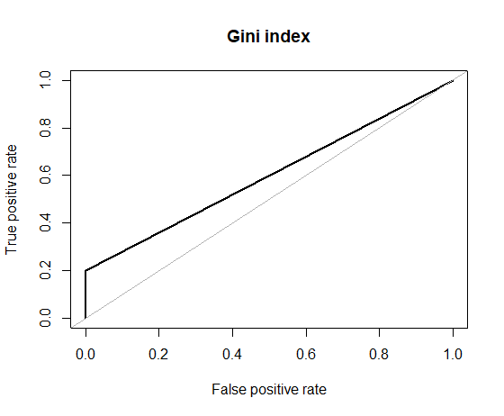
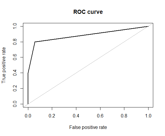
# F: 0.167

Things don’t look all that great. Although we have a perfect precision (reminder: Precision=TP/(TP+FP)), meaning that we don’t have any false positives, our recall is very low (reminder: Recall=TP/(TP+FN), meaning that we have many false negatives. So basically, our classifier outputs pretty much always the majority class “0”. F-metric also is very low. And this is the ROC curve which shows how horrible our performance is.

roc.curve(hacide.test$cls, pred.tree.imb[,2], plotit = T, main = "Gini index")
# Area under the curve (AUC): 0.600

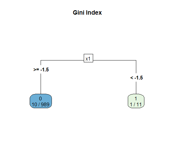
So what did go wrong here? Let’s take a look at the decision tree itself. Notice that the left node has 10 observations of the minority class and 979 of the dominant class. From the perspective of Gini impurity index that’s a very pure node, because \(G_L = 1 - (10/989)^2 - (979/989)^2 \simeq 0.02\). The same applies, albeit to a lesser degree, for the right node: \(G_R = 1 - (1/11)^2 - (10/11)^2\simeq 0.17\). Therefore, \(G\) doesn’t appear to be working so great with our imbalanced dataset.

rpart.plot(tree.imb, main = "Gini Index", type = 5, extra = 3)

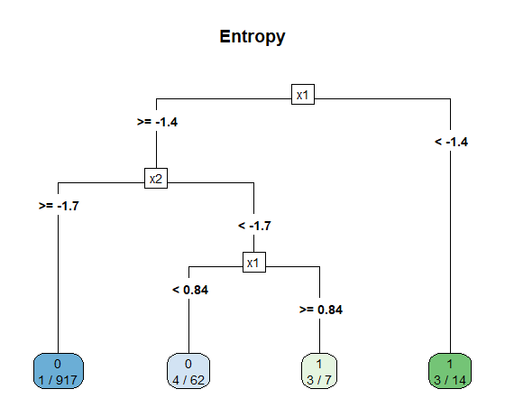
Let’s repeat the fitting, but now we will use entropy as the split criterion for growing our tree.

# Use information gain as the split criterion
tree.imb <- rpart(cls ~ ., data = hacide.train, parms = list(split = "information"))
pred.tree.imb <- predict(tree.imb, newdata = hacide.test)
accuracy.meas(hacide.test$cls, pred.tree.imb[,2])
#
# Call: 
# accuracy.meas(response = hacide.test$cls, predicted = pred.tree.imb[, 2])
#
#  Examples are labelled as positive when predicted is greater than 0.5 
#
# precision: 1.000
# recall: 0.400
# F: 0.286

The precision is still perfect, i.e. we aren’t predicting any false positives, and we doubled the recall. This improvement also reflects to the F metric. Also, the ROC curve of the new decision tree is way better than the previous run.

roc.curve(hacide.test$cls, pred.tree.imb[,2], plotit = T)
# Area under the curve (AUC): 0.883

Here is the decision tree itself. Admittedly, it’s a bit more complex that when we used Gini, but overall the classifier is more performant and useful.

rpart.plot(tree.imb, main = "Information Gain", type = 5, extra = 3)