The meaning of curl operator
mathematics physics vector analysisContents
Introduction
Quoting the wikipedia definition of the curl vector operator:
In vector calculus, the curl is a vector operator that describes the infinitesimal rotation of a vector field in three-dimensional Euclidean space. At every point in the field, the curl of that point is represented by a vector. The attributes of this vector (length and direction) characterize the rotation at that point.
The devil in this definiton lies in the word infinitestimal. I was under the impression that curl was related to the macroscopic rotation, but I couldn’t be more wrong! Let me show what I mean. Consider the vector field defined by \(\mathbf{F}(x,y,z) = \left(-y/(x^2+y^2), x/(x^2+y^2), 0\right)\).
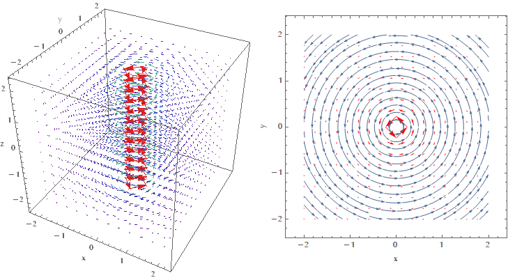
By looking at these images my first reaction was that this field is most certainly a rotational one. I mean look at how “swirly” it is! Imagine my surprise when I actually did the math and my intuition proved to be completely wrong:
\[\begin{align} \nabla \times \mathbf{F} &= \begin{vmatrix} \mathbf{i} & \mathbf{j} & \mathbf{k} \\[5pt] {\dfrac{\partial}{\partial x}} & {\dfrac{\partial}{\partial y}} & {\dfrac{\partial}{\partial z}} \\[10pt] F_x & F_y & F_z \end{vmatrix}\\ &= \left(\frac{\partial F_z}{\partial y} - \frac{\partial F_y}{\partial z}\right) \mathbf{i} + \left(\frac{\partial F_x}{\partial z} - \frac{\partial F_z}{\partial x} \right) \mathbf{j} + \left(\frac{\partial F_y}{\partial x} - \frac{\partial F_x}{\partial y} \right) \mathbf{k}\\ &= (0 - 0)\mathbf{i} + (0 - 0) \mathbf{j} + \left[\frac{-x^2+y^2}{(x^2+y^2)^2} - \frac{-x^2+y^2}{(x^2+y^2)^2}\right] \mathbf{k} = \vec{0} \end{align}\]How can it be that this plot corresponds to an irrotational field? Well, it depends on which rotation you are referring to (macroscopic vs. microscopic or global vs. local). Curl measures the local rotation! Imagine that this vector field describes the flow of water in a pool with a sink at the bottom that sucks the water out it. If we put a small ball on the surface of the water, then the ball may move in two distinct ways:
- The general rotation of the flow around the z-axis (z-axis is perpendicular to your monitor) in the counterclockwise direction, along the direction of the stream lines (blue arrows).
- Since the arrows of the field are longer the closer we are to the z-axis, the field tends to push the ball more strongly on the side closest to the z-axis, rather than the opposite side. The “differential” push on the two sides of the ball would tend to make it rotate around itself in the clockwise direction.
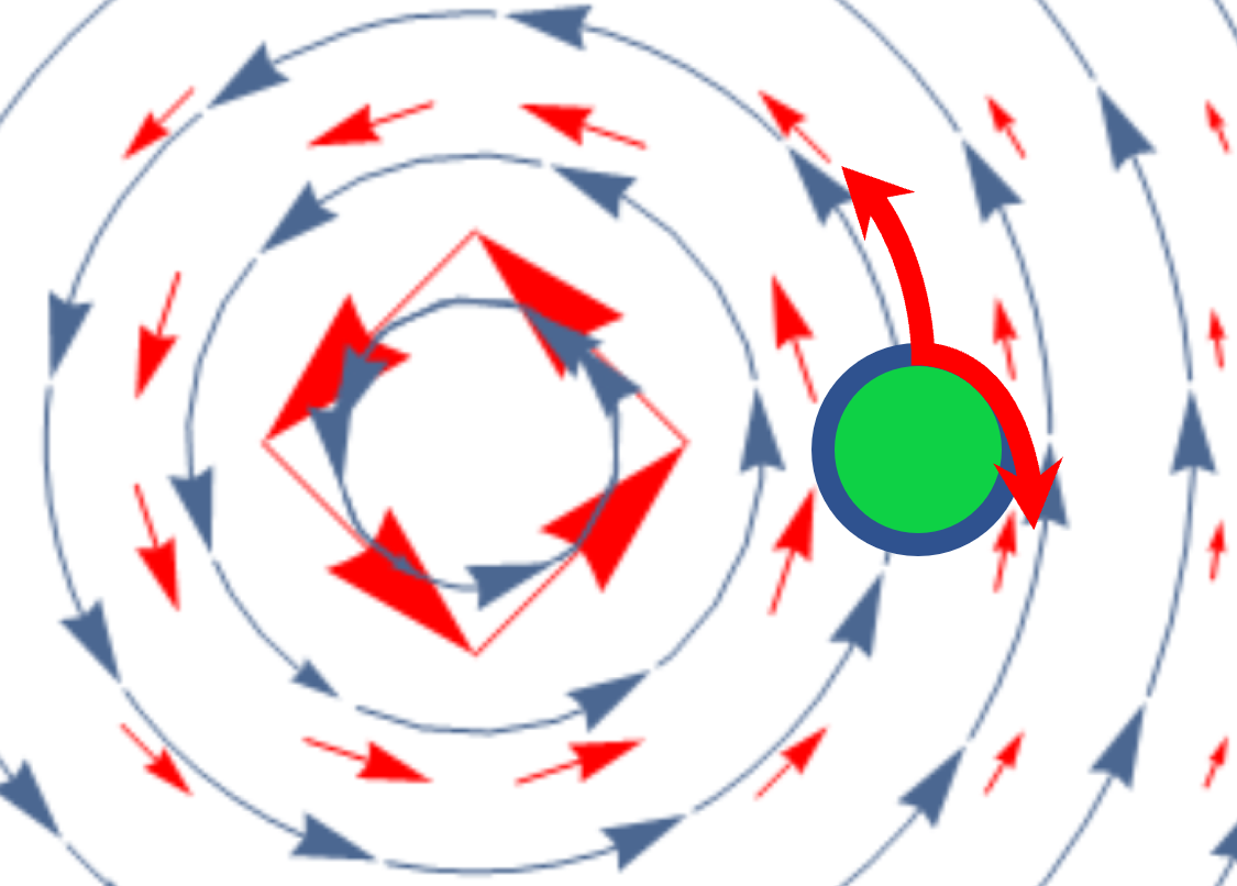
These two opposite effects may cancel out (as in our case) and then the curl is zero. The ball still moves inside the pool around the z-axis, but it doesn’t rotate around itself, which is what the curl operator measures.
Another way to view curl
Please mind that the image above is drawn in a large scale. In reality the green circle is infinitestimal. Another way to look at curl is as the average circulation of a field in a region that shrinks around a point, i.e.:
\[\lim_{A\to 0} \left( \frac{1}{A} \oint_C \mathbf{F} \cdot \operatorname{d}\! \mathbf{r} \right)\]Where \(A\) is the green area in the image above, as it shrinks into a point. Recall though that the curl is a vector, so the correct way to connect the above formula with the curl is:
\[(\nabla \times \mathbf{F}) \cdot \hat{\mathbf{n}} = \lim_{A\to 0} \left( \frac{1}{A} \oint_C \mathbf{F} \cdot \operatorname{d}\!\mathbf{r} \right)\]where \(\hat{\mathbf{n}}\) is the normal vector to the point \(O\) where we measure the curl.
Relation of curl with the angular velocity at some point
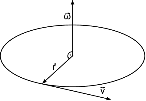
By now, it shouldn’t come as a surprise that the curl of a vector field calculated at some point \(O\), is related to the angular velocity of a rotating object with its center fixed at \(O\). Let’s do the math!
First method
Let us calculate the curl of \(\mathbf{v}\):
\[\nabla \times \mathbf{v} = \begin{vmatrix} \mathbf{i} & \mathbf{j} & \mathbf{k} \\[5pt] {\dfrac{\partial}{\partial x}} & {\dfrac{\partial}{\partial y}} & {\dfrac{\partial}{\partial z}} \\[10pt] \nu_x & \nu_y & \nu_z \end{vmatrix}\]The \(x\) component of \(\nabla \times \mathbf{v}\) is (for brevity we write \(\partial_x\) instead of \({\partial}/{\partial_x}\)):
\[\left( \nabla \times \mathbf{v} \right)_x = {\partial_y \nu_z} - {\partial_z \nu_y}\]Recall though that \(\mathbf{v} = \boldsymbol{\omega} \times \mathbf{r} \Rightarrow \nu_z = \omega_x y-\omega_y x\) and similarly \(\nu_y = \omega_x z - \omega_z x\). Therefore:
\[\begin{align} \left( \nabla \times \mathbf{v} \right)_x &= {\partial_y \nu_z} - {\partial_z \nu_y}\\ &= \partial_y (\omega_x y - \omega_y x)- \partial_z (\omega_x z - \omega_z x)\\ &= \omega_x + \omega_x = 2\omega_x \end{align}\]Similarly it is \(\left( \nabla \times \mathbf{v} \right)_y = 2 \omega_y\) and \(\left( \nabla \times \mathbf{v} \right)_z = 2\omega_z\). Therefore the curl is twice the angular velocity:
\[\nabla \times \mathbf{v} = 2 \boldsymbol{\omega}\]Second method
Another way to attack the problem is by calculating the average circulation of the vector field \(\mathbf{v}\) around the point \(O\). For simplicity let us assume that we are working on a vector field in two dimensions (\(xy\) plane):
\[\begin{align*} \mathbf{v} &= \boldsymbol{\omega} \times \mathbf{r} = \begin{vmatrix} \mathbf{i} & \mathbf{j} & \mathbf{k} \\[5pt] {\omega_x} & {\omega_y} & {\omega_z} \\[10pt] x & y & z \end{vmatrix} = \begin{vmatrix} \mathbf{i} & \mathbf{j} & \mathbf{k} \\[5pt] {0} & {0} & {\omega_z} \\[10pt] x & y & z \end{vmatrix}\\ &= (-\omega_z y)\mathbf{i} - (- \omega_z x) \mathbf{j} = -\omega_z y\mathbf{i} + \omega_z x \mathbf{j} \end{align*}\] \[I = \oint_C \mathbf{v} \cdot \operatorname{d}\!\mathbf{r} = \oint_C (\boldsymbol{\omega} \times \mathbf{r}) \cdot \operatorname{d}\!\mathbf{r} = \oint_C(-\omega_z y\mathbf{i} + \omega_z x \mathbf{j}) \cdot \operatorname{d}\!\mathbf{r}\]We use the parameterization \(\mathbf{r}(t) = \rho \cos t \mathbf{i} + \rho \sin t \mathbf{j} \Rightarrow \mathbf{r}'(t) = -\rho \sin t \mathbf{i} +\rho \cos t \mathbf{j}\), with \(t = [0, 2\pi]\).
Therefore:
\[\begin{align*} I &= \int_0^{2\pi} (-\omega_z \rho \sin t\mathbf{i} + \omega_z \rho \cos t \mathbf{j}) \cdot (-\rho \sin t \mathbf{i} + \rho \cos t \mathbf{j}) \operatorname{d}\!t\\ &= \int_0^{2\pi} \omega_z \rho^2 \sin^2 t + \omega_z \rho^2 \cos^2 t \operatorname{d}\!t \\ &= \int_0^{2\pi} \omega_z \rho^2 \operatorname{d}\!t = 2\pi\rho^2 \omega_z \end{align*}\]Therefore:
\[(\nabla \times \mathbf{v}) \cdot \hat{\mathbf{n}} = \lim_{A\to 0} \left( \frac{1}{A} \oint_C \mathbf{v} \operatorname{d}\!\mathbf{r} \right) = \lim_{\rho \to 0} \left( \frac{1}{\pi \rho^2} 2\pi \rho^2 \omega_z\right) = 2\omega_z\]