Arcsin transformation gone wrong
machine learning mathematics neural networksSo, I was working on a regression problem and my \(y\) values, in theory, would fall in the range \([0,1]\). In reality, though, most of them were crowded between \(0.9\) and \(1.0\). I thought that I could apply some transformation and distribute them more evenly, without thinking about it too much.
Therefore, I applied the arc sine square transformation, again, without checking when this transformation would make sense.
\[z = \text{arcsin}(\sqrt{y})\]After running my code to the transformed data set, I noticed that not only did the model not perform better, but the results I was getting were very bad.
The reason behind this failure is, I guess, that my data were noisy and this transformation inflated the error. You can check this wikipedia article on propagation of uncertainty. A common formula to calculate error propagation is the following. Assuming that you have \(z = f(x, y, \ldots)\), then your error in the variable \(z\) is given by:
\[s_z = \sqrt{ \left(\frac{\partial f}{\partial x}\right)^2 s_x^2 + \left(\frac{\partial f}{\partial y} \right)^2 s_y^2 + \cdots}\]Where \(s_z\) represents the standard deviation of the function \(f\), \(s_x\) represents the standard deviation of \(x\), \(s_y\) represents the standard deviation of \(y\) and so forth.
So, in my case it was simply this:
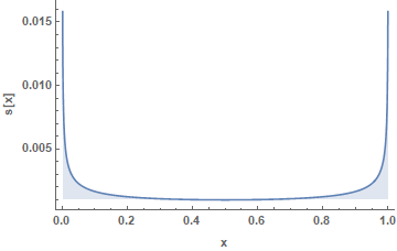
\[s_z = \frac{\mathrm{d} z}{\mathrm{d} y} s_y \Rightarrow s_z = \frac{1}{2\sqrt{y (1-y)}} s_y\]And since my \(y\)’s were very close to \(1\), naturally \(s_z\) exploded.
Moral: don’t try random stuff; make educated guesses.
Excercise for the reader: What data transformation would actually reduce my error? Can you think of some function \(z = f(y)\), such as that when you calculate \(\frac{\mathrm{d} z}{\mathrm{d} y}\), \(s_z\) is smaller compared to \(s_y\) for \(y\) values close to \(1\)?