An almost one-liner to construct the Mandelbrot set with Mathematica
complex numbers fractals functional programming Mathematica mathematics programmingThe motivation
Benoit Mandelbrot was a mathematician best known for the discovery of fractal geometry and the famous homonymous set. Mandelbrot was born on 20 November 1924, and I was hoping to honor his birthday by writing a short post for the Mandelbrot set. However, I missed the date because I was working on my master thesis. Anyway, even though I am off by a few days, let’s do it!

Source: Photo attributed to Soo Jin Lee.
The definition
Mandelbrot set is the set of all complex numbers \(c\) that fulfill the following condition:
\[z_{n+1} = z^2_n + c, \text{does not diverge, starting with } z_0 = 0\]
So for every point in the complex plane \(\mathbb{C}\), we assume the complex number \(c = a + b i, \, a,b\in\mathbb{R}\) and then we calculate the infinite series:
\[\underbrace{c}_{z_1}, \,\,\underbrace{c^2+c}_{z_2}, \,\,\underbrace{(c^2+c)^2+c}_{z_3}, \,\,\underbrace{((c^2+c)^2+c)^2+c}_{z_4}, \ldots\]If this series doesn’t diverge, then \(c\) belongs to the Mandelbrot set. If it diverges, then it does not belong to the set. In practice, we only calculate a finite number of terms, e.g., 256 or whatever. And we color the point \(c\) according to the number of iterations that we had to go through before we could tell whether it diverged or not.
For example, let us check whether \(c=1+i\) is an element of the Mandelbrot set or not. We calculate the sequence \(z_1, z_2, \ldots\) and notice that \(z_1 = 1+i\), and \(\|1+i\|=\sqrt{1^2+1^2}=\sqrt{2} < 2\). We proceed to the next term of the sequence, with \(z_2 = (1+i)^2 + (1+i) = 1 + 2i + i^2 + 1 + i = 1 + 3i\). But, \(\|1+3i\|= \sqrt{1^2+3^2} = \sqrt{10} > 2\). Therefore, the series diverges, and the complex number \(1+i\) does not belong to the set. We figured this out with only 2 iterations, therefore we would color this point of complex plane with the “2nd color” of our palette.
The almost one-liner
In the following code, \(f[c\_]\) checks whether \(c\) belongs to the Mandelbrot set or not. If it does not, it returns the number of iterations needed to reach this conclusion. If we perform 255 iterations, we assume that the series doesn’t diverge, and we take \(c\) to belong to the set.
f[c_] := NestWhileList[#^2 + c &, c, Abs[#] <= 2. &, 1, 255] // Length
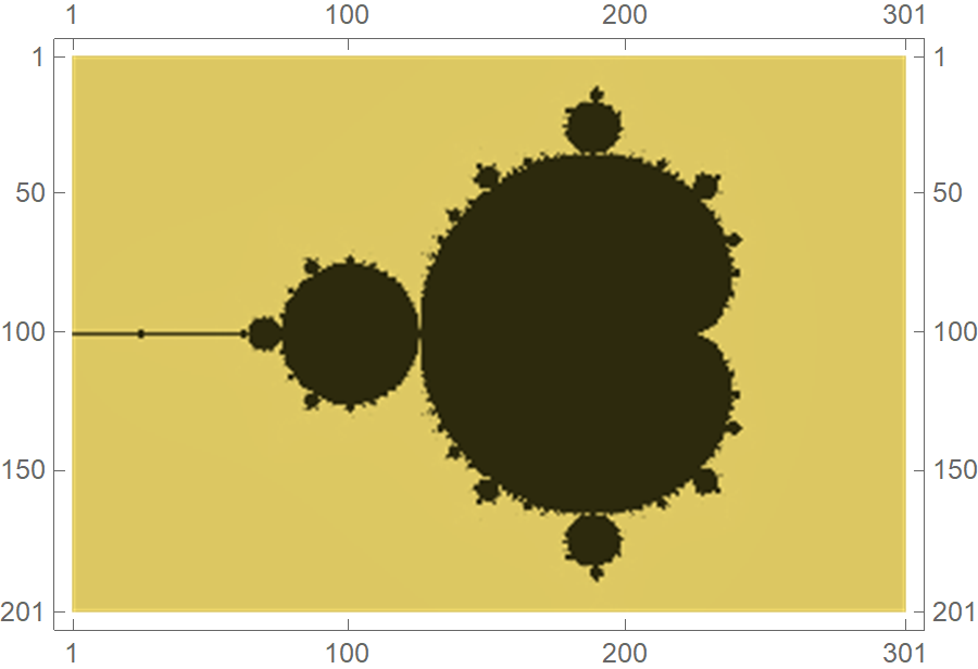
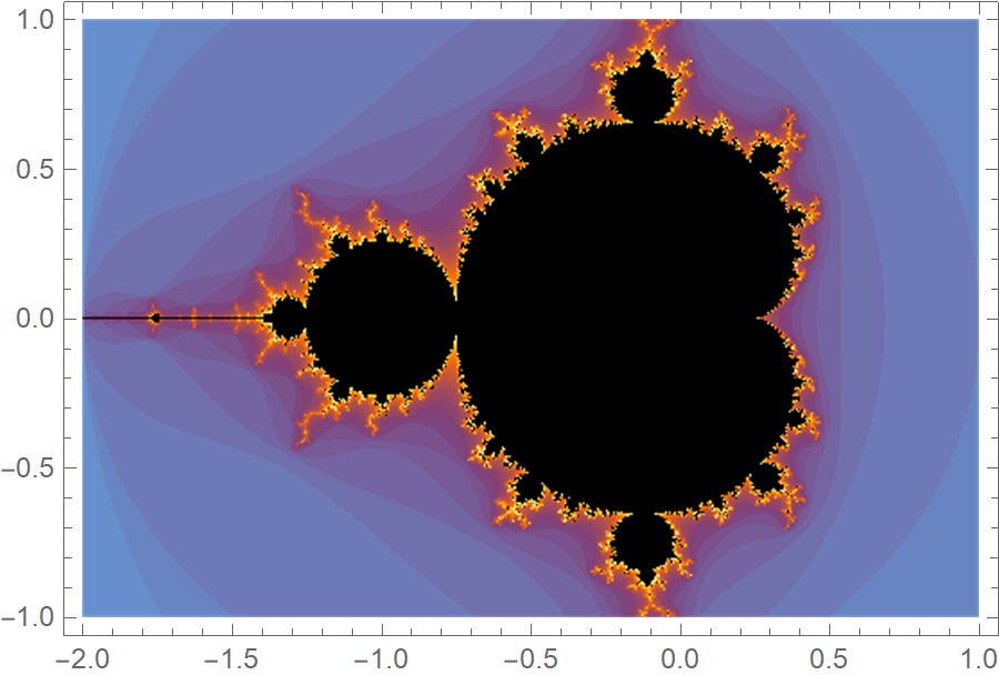
mandel[res_] := Transpose@ParallelTable[f[x + y I], {x, -2., 1, res}, {y, -1, 1, res}];
MatrixPlot[mandel[0.01], ColorFunction -> "BrassTones"]
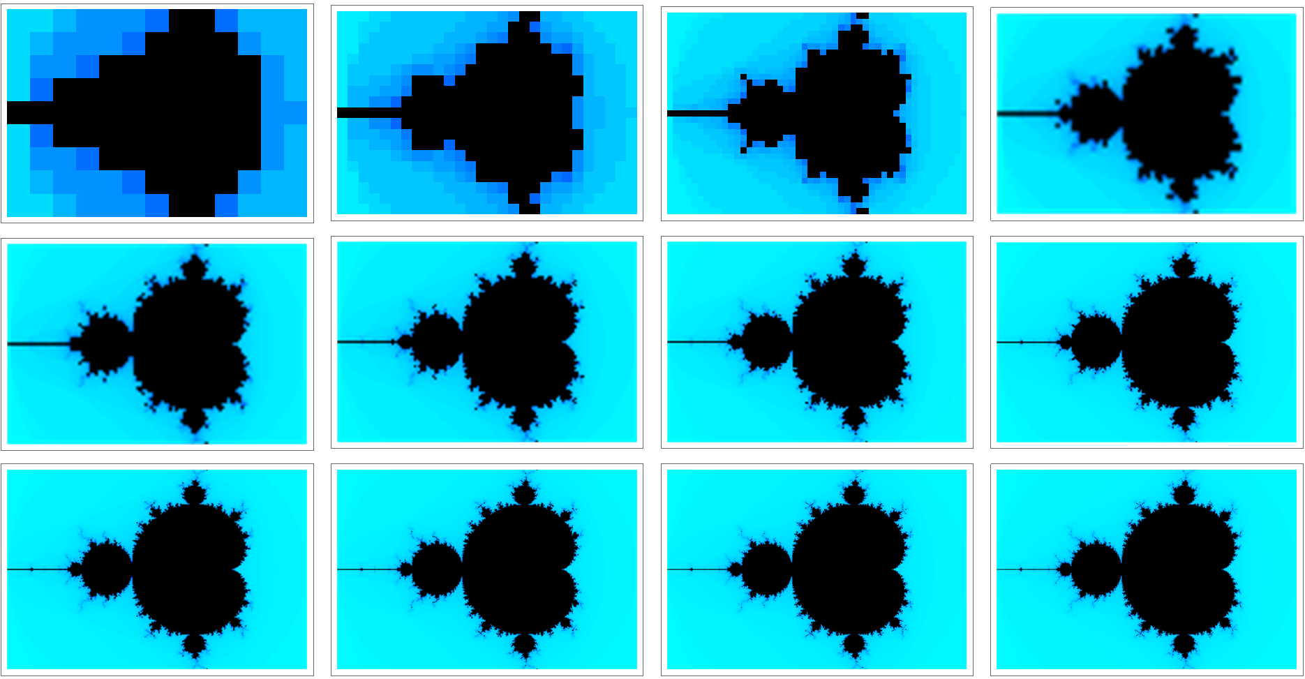
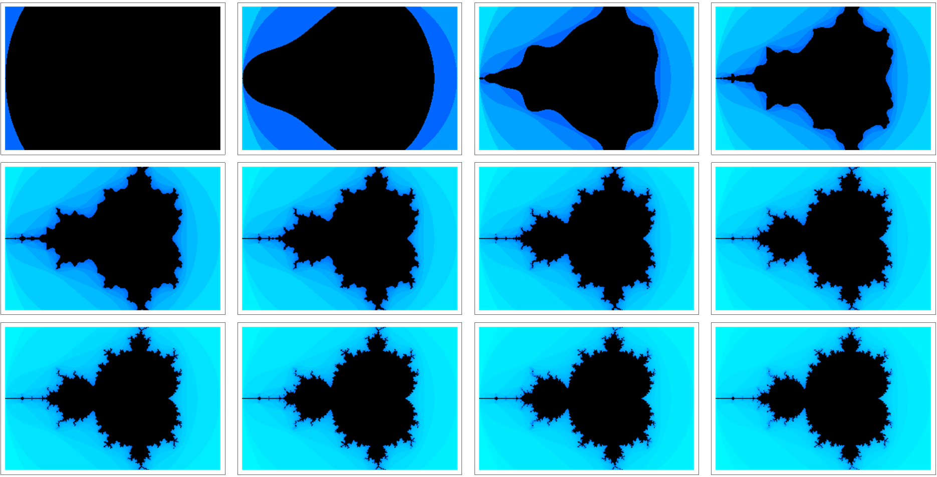
The following code visualizes the set with increasing resolution. As we scan the complex plane \(\mathbb{C}\) with a finer resolution, the set’s boundary gets increasingly intricate.
Table[
    MatrixPlot[mandel[1/k^2],
        ColorFunction -> Function[x, If[x > 0.6, Black, Hue@x]], FrameTicks -> None],
    {k, 2, 13}]
And by tweaking the code a bit, we can visualize the Mandelbrot set while increasing the maximum iterations threshold.
The explanation
Recall that we want to calculate the infinite series \(f(0), f(f(0)), f(f(f(0))), \ldots\), where \(f(x) = x^2 + c\). In Mathematica, there’s the function Nest[] that applies iteratively a function to some given expression and returns the result:
Clear[f];
Nest[f,x,5]
(* f[f[f[f[f[x]]]]] *)
However, we would like to accumulate the intermediate results so that we can count them and check if we have reached the maximum number of iterations. Therefore, we would need something like:
Table[
 Nest[f, x, k],
 {k, 0, 3}]
(* {x, f[x], f[f[x]], f[f[f[x]]]} *)
Fortunately, Mathematica has NestList[] that does precisely this!
NestList[f, x, 3]
(* {x, f[x], f[f[x]], f[f[f[x]]]} *)
We are almost there, but how can we check whether in each iteration the absolute value of the complex number is less than 2? We need a NestList[] function that allows us to inject some sort of condition. Enter NestListWhen[]!
With[{c = 1 + I},
 NestWhileList[#^2 + c &, c, Abs[#] <= 2 &, 1, 255]
]
(* {1 + I, 1 + 3 I} *)
It is now evident what \(f[c\_]\) does in the one-liner. It applies the lambda function #^2 + c iteratively to the previous result, starting with \(z_1 = c\). At each iteration, it checks whether the absolute value of current \(z_{n+1}\) is less or equal to 2. If it is, it continues the iterative process. If it’s not, it terminates the loop and counts the number of intermediate computations we performed with Length[]. Isn’t functional programming fantastic?
The (no pun intended) plot twist
Up until know we considered the infinite series of \(z_{n+1} = z_n^2 + c, c\in\mathbb{C}\), where \(z_0\) was fixed to zero and \(c\) scanned the complex plane. What if we fix \(c\) to some complex number and let \(z_0\) scan the complex plane? This is left as an excercise to the reader, but for \(c=i\), you should get something along the lines of the following plot:
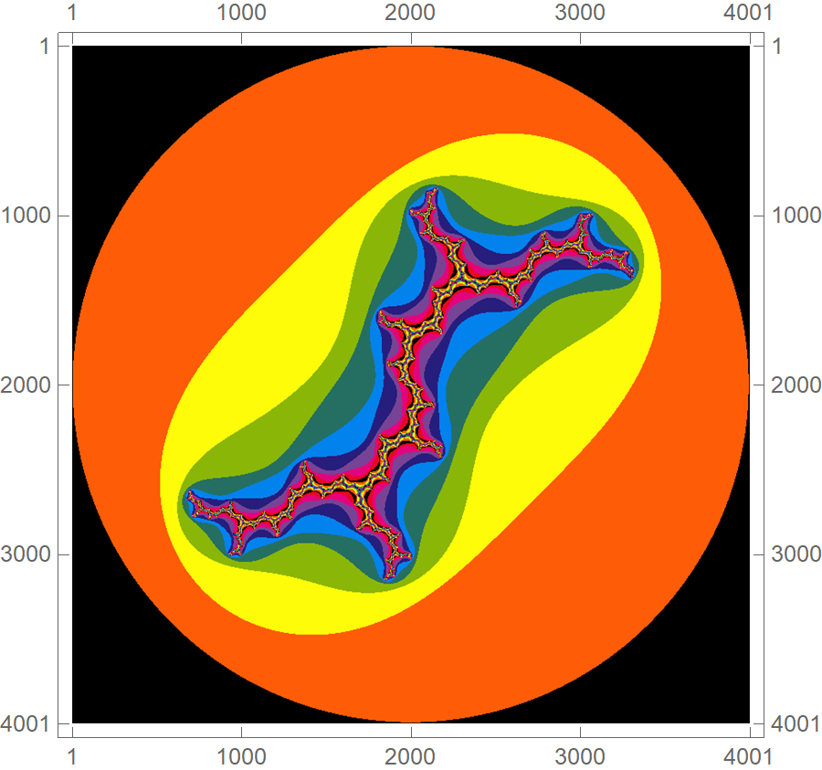
Congratulations! You have just discovered the Julia set!
The mind-blowing
You might be thinking that keeping track of intermediate computations in NestedWhileList[] is a waste of resources. In some sense, it is, if we only want to plot the Mandelbrot set. However, we could plot all the intermediate elements of the recursion \(z \mapsto z^2 + c\). For many points \(c\) of the complex plane \(\mathbb{C}\), nothing special happens. For other points, though, some very cool patterns emerge. Here is a snapshot.
p1 = MatrixPlot[mandel[0.01], ColorFunction -> "BrassTones", ImageSize -> Large, Frame -> False]

plotCourse[c_] :=
 Module[{pts, pts2},
  pts = NestWhileList[#^2 + c &, c, Abs[#] <= 2 &, 1, 255];
  pts2 = {Re@#, Im@#} & /@ pts;
  ListPlot[pts2, PlotStyle -> {Red, PointSize[0.005]},
   PlotRange -> {{-2, 1}, {-1, 1}}, Prolog -> Inset@p1,
   ImageSize -> Large, PlotRangeClipping -> True]
  ]

  plotCourse[0.16 - 0.57 I]
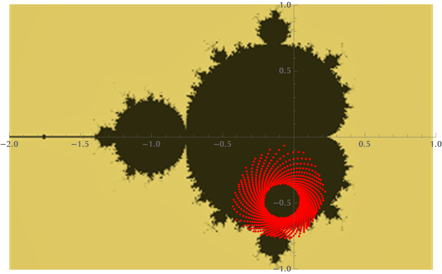
And here is a video of drawing the intermediate points in the complex plane. Every sequence starts with \(c\) being equal to the point the mouse cursor is at. Notice that interesting patterns arise when we hover the mouse near the boundary of the set.
The intuition
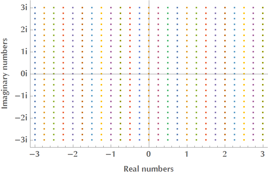
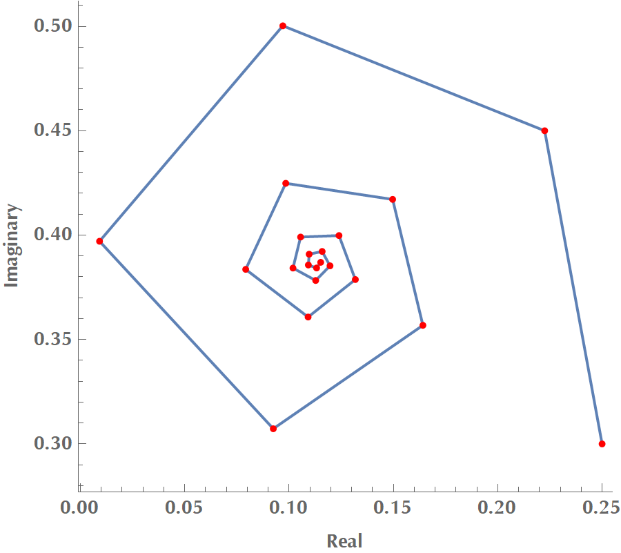
In the following figure, we see the effect of starting with \(c = 0.3 + 0.25i\) and calculating the series \(z_{n+1} = z_n^2 + c\). Every red dot is a complex number corresponding to \(z_1, z_2, z_3, \ldots, z_{21}\). In this case, the series converges spiraling towards a vanishing polygon.
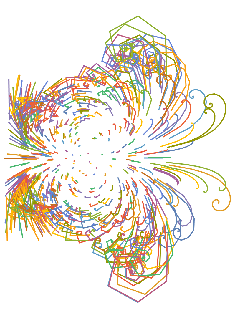
In this figure, we do the same as before, but we superimpose the orbits of hundreds starting points in the complex plane, corresponding to many different \(c\) numbers. You may even “see” the blueprint of the Mandelbrot set if you stare at it for a bit.
Let’s see what happens when we square a complex number \(z\). In this context, we will represent \(z\) in polar form, i.e. \(z=r e^{i\theta}\):
\[z = r e^{i\theta} \Rightarrow z^2=(re^{i\theta})(re^{i\theta})=r^2e^{2i\theta}=r^2e^{i(2\theta)}\]It’s evident now that squaring a complex number is equivalent to scaling its magnitude and rotating it. Also, adding a complex number \(c\) to \(z\), is equivalent to translating \(z\). Therefore, the sequence:
\[\underbrace{c}_{z_1}, \,\,\underbrace{c^2+c}_{z_2}, \,\,\underbrace{(c^2+c)^2+c}_{z_3}, \,\,\underbrace{((c^2+c)^2+c)^2+c}_{z_4}, \ldots\]could be viewed as an infinite series of scale, rotate, translate operations:
\[\underbrace{c}_{z_1}, \,\,\underbrace{\text{scale-rotate-translate }z_1}_{z_2}, \,\,\underbrace{\text{scale-rotate-translate }z_2}_{z_3},\ldots\]The nitpicker
There’s actually a built-in command in Mathematica 10.0 that plots the Mandelbrot set, so you could really construct it with one-line!
MandelbrotSetPlot[{-2 - I, 1 + I}, MaxIterations -> 50]
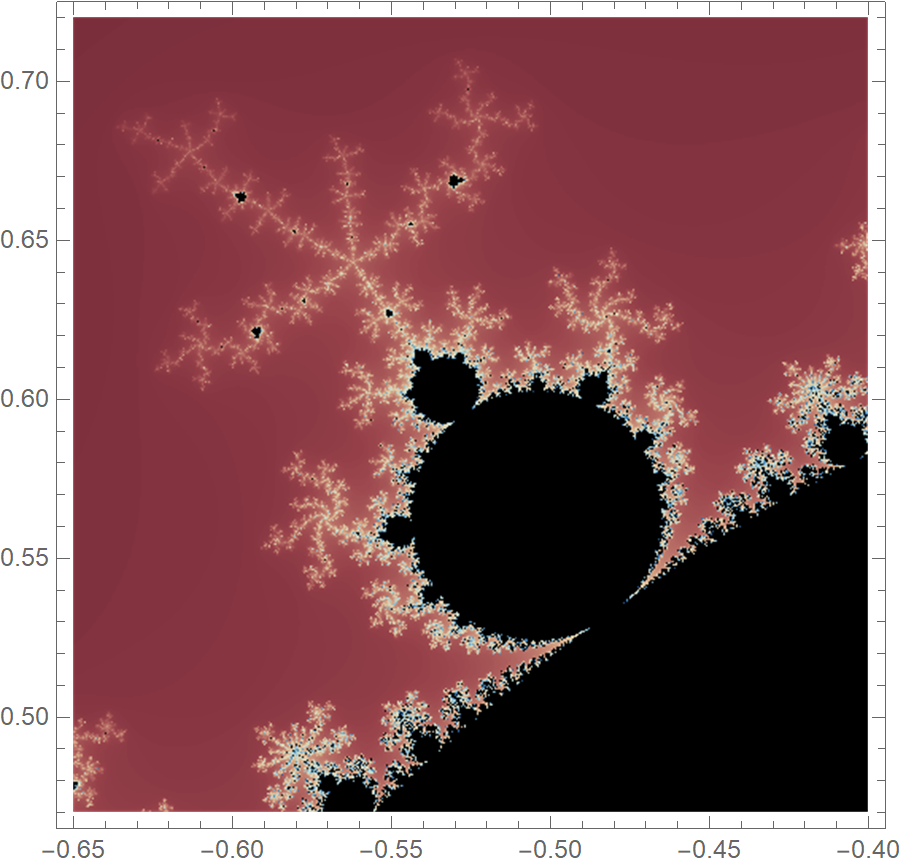
MandelbrotSetPlot[{-0.65 + 0.47 I, -0.4 + 0.72 I},
 MaxIterations -> 200, ColorFunction -> "RedBlueTones"]