A gentle introduction to kernel density estimation
Mathematica mathematics statisticsIntroduction
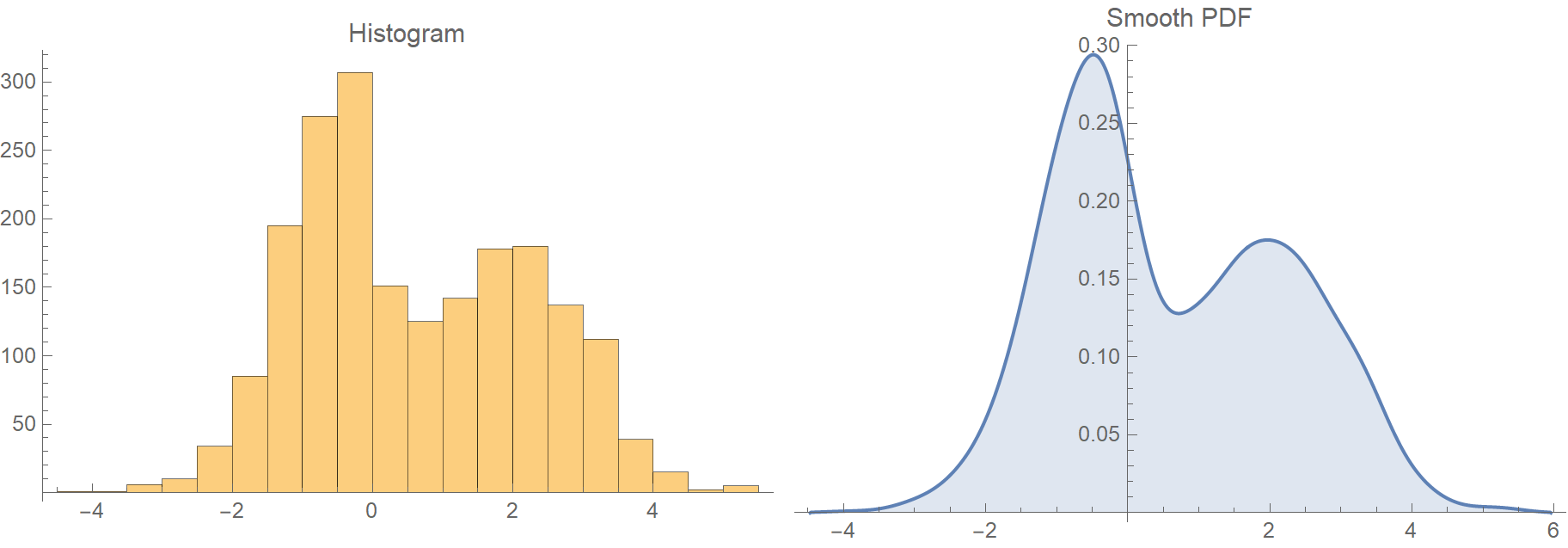
Suppose we have some low dimensional data (1 or 2 variables). How do we start exploring them? Usually, one of the first steps is to plot their histogram to get a feeling of how they are distributed. Histograms are nice because they provide a fast and unambiguous way to visualize our data’s probability distribution. However, they are discrete, and sometimes it is useful to have a smooth estimation of the underlying probability density function (PDF) at hand.
There are two ways to get a smooth PDF from your data.
- The parametric probability density estimation where we pick a common distribution (say a normal distribution), and we estimate its parameters (e.g., mean, standard deviation) from the data sample.
- The nonparametric probability such as kernel density estimation (KDE), that we will be discussing today.
The case of 1 variable
In the univariate case, that is when we have only one variable, KDE is very straightforward. Here is how we’d do it. Assuming we have a set of \(N\) samples \(x_i = \{x_1, x_2, \ldots, x_N\}\), the KDE, \(\hat{f}\), of the PDF is defined as:
\[\hat{f}(x,h) = \frac{1}{N} \sum_{i=1}^{N} K_h (x-x_i)\]Basically, in the kernel density estimation approach, we center a smooth scaled kernel function at each data point and then take their average. One of the most common kernels is the Gaussian kernel:
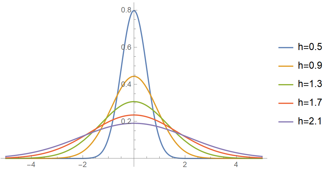
\[K(u)\text = \frac{1}{\sqrt{2 \pi}} \exp \left(-\frac{u^2}{2}\right)\\\]The \(K_h\) is the scaled version of the kernel, i.e., \(K_h(u) = \frac{1}{h} K\left(\frac{u}{h}\right)\). The parameter \(h\) of the kernel is called the bandwidth, and this little number is a very critical determinant of our estimate’s quality. As important as the kernel choice itself! By tweaking its value, we change the width of the kernel as in the next figure:
Here is a concrete example that sums all of the above:
ClearAll["Global`*"];

(* Assume some sample data *)
pts = {1, 2, 3, 4, 7, 9};

(* Define the kernel *)
k[u_] := 1/Sqrt[2 Pi] Exp[-u^2/2]
k[h_, u_] := 1/h k[u/h]

(* Define the kernel density estimate *)
f[x_, h_] :=
 With[{n = Length@pts}, 1/n Sum[k[h, x - pts[[i]]], {i, 1, n}]] // N

(* Get a kernel density estimate for bandwidth equal to one *)
f[x, 1]
And this is the output:
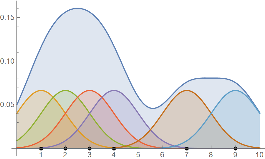
\[\begin{align*} \hat{f}(x,1) = \frac{1}{6} \left(\frac{e^{-\frac{1}{2} (x-9)^2}}{\sqrt{2 \pi }}+\frac{e^{-\frac{1}{2} (x-7)^2}}{\sqrt{2 \pi }}+\frac{e^{-\frac{1}{2} (x-4)^2}}{\sqrt{2 \pi }}+\frac{e^{-\frac{1}{2} (x-3)^2}}{\sqrt{2 \pi }}+\frac{e^{-\frac{1}{2} (x-2)^2}}{\sqrt{2 \pi }}+\frac{e^{-\frac{1}{2} (x-1)^2}}{\sqrt{2 \pi }}\right) \end{align*}\]In the following figure, we plot both the individual Gaussian kernels, along with the kernel density estimate. The black dots are our data points and notice how they are at the kernels’ center.
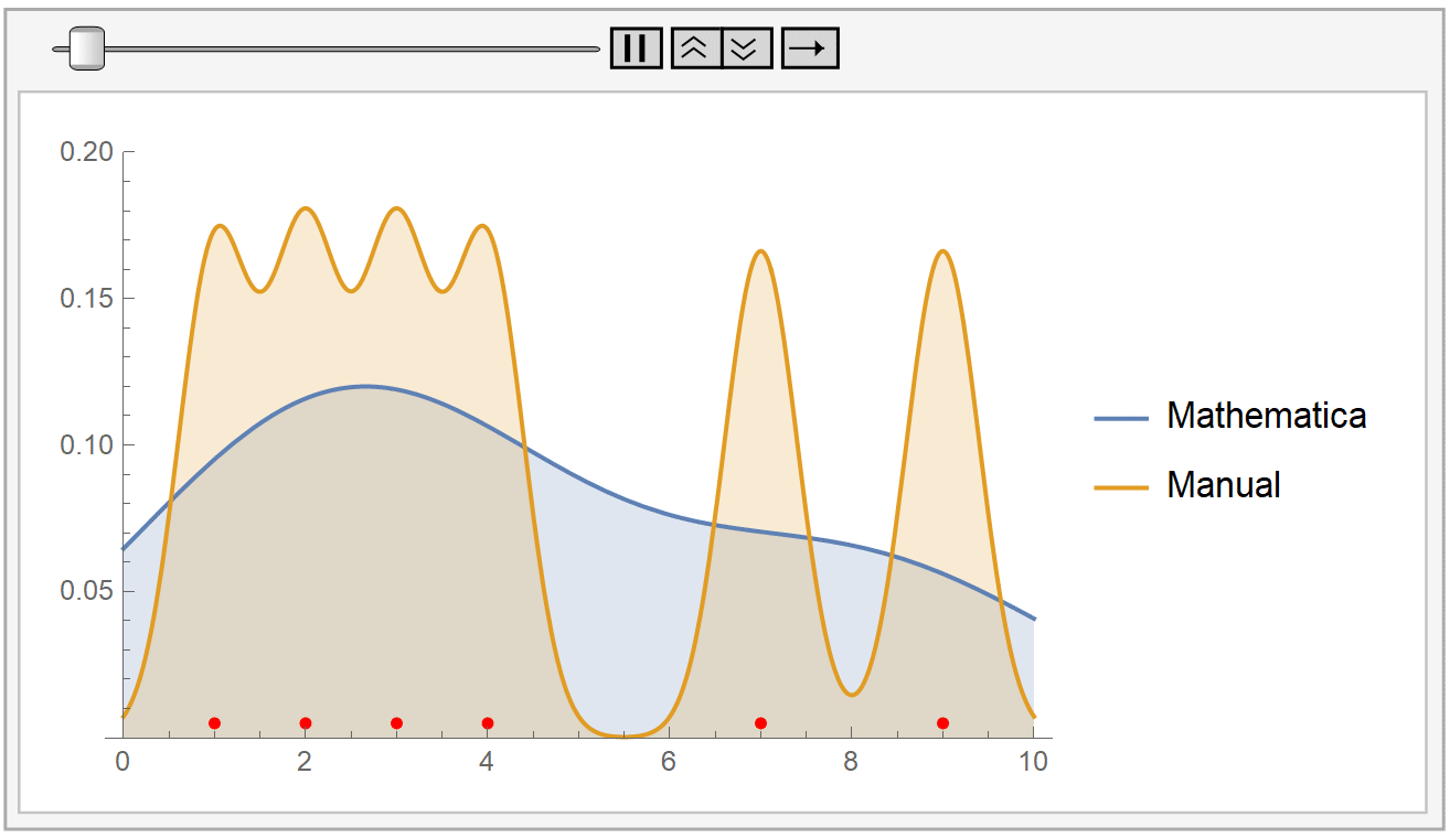
In the following animation, we plot the output of Mathematica’s built-in SmoothKernelDistribution[] function and our own kernel density estimation for varying values of the bandwidth parameter \(h\). The red dots at the bottom represent our sample data, the same as before. Notice how for small values of the bandwidth parameter \(h\) (during the start of the animation), the KDE is rigged. But, as \(h\) increases, the estimate gets smoother and smoother. The selection of the parameter \(h\) is, as we have already said, very crucial.
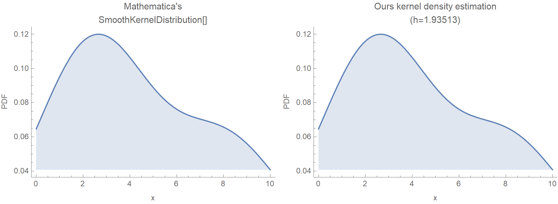
Mathematica uses the Silverman’s rule of thumb for bandwidth estimation, via the following formaula:
\[h = 0.9\, \min\left(\hat{\sigma}, \frac{\text{IQR}}{1.34}\right)\, n^{-\frac{1}{5}}\]In our case it is:
sigma = StandardDeviation[pts];
iqr = InterquartileRange[pts];
n = Length[pts];
0.9 Min[sigma, iqr/1.34]*n^(-1/5)

(* 1.93513 *)
Unless we have screwed things up, if we pass \(h = 1.93513\) to our KDE, we should get an identical result compared to Mathematica.
Grid[{
  Plot[Last@#, {x, 0, 10}, Frame -> {True, True, False, False},
     FrameLabel -> {"x", "PDF"}, ImageSize -> Medium,
     PlotLabel -> First@#, Filling -> Axis] & /@ {
    {"Mathematica's\nSmoothKernelDistribution[]", PDF[SmoothKernelDistribution[pts], x]},
    {"Ours kernel density estimation\n(h=1.93513)", f[x, 1.93513]}}
  }]
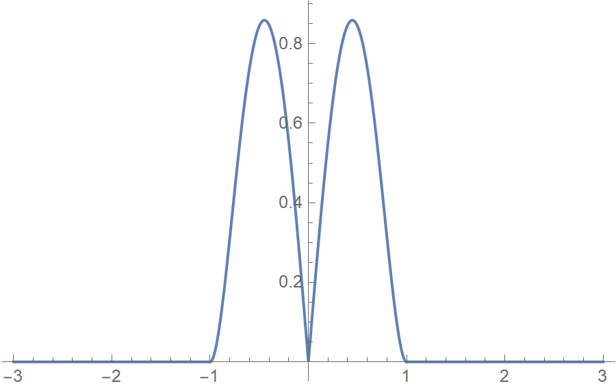
In principle, we could use whatever kernel we’d like, as long as it is symmetric, non-negative, and integrates to 1. However, our choice should take into consideration the underlying process that generates our data. In the following example, we use a bisquare kernel on the same data as before.
The bisquare kernel is symmetric, non-negative, and integrates to 1.
\[K(u) = (1-u^2)^2 |u| \mathbf{I}_{\{|u|<1\}} \hspace{2cm} K(u) \ge 0, u \in \mathbb{R} \hspace{2cm} \int_{-\infty}^{\infty} K(u) \mathrm{d}u =1\]ind[u_] := If[Abs[u] < 1, 1, 0];
k2[u_] := 3 (1 - u^2)^2*Abs[u] ind[u]
Plot[k2[u], {u, -3, 3}, PlotRange -> All]
k2[h_, u_] := 1/h k2[u/h]
Integrate[k2[u], {u, -Infinity, Infinity}]
(* 1 *)
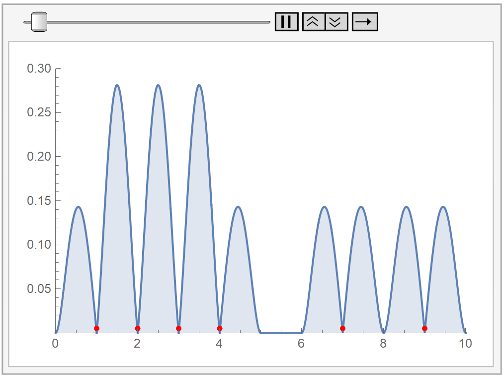
In the following animation, we plot our own kernel density estimation for varying bandwidth parameter values \(h\). The red dots at the bottom represent our sample data, the same as before.
Kernel density estimation has two difficulties:
- Optimal bandwidth estimation.
- The varying data density makes regions of high data density requiring small bandwidths, and areas with sparse data needing large bandwidths.
The case of 2 variables
The bivariate kernel density estimate is defined in a similar manner:
\[\hat{f}(\mathbf{x}, \mathbf{H}) = \frac{1}{N}\sum_{i=1}^N K_{\mathbf{H}} \left(\mathbf{x} - \mathbf{x}_i\right)\]Since we are in two dimensions, our \(\mathbf{x}\)’s are tuples \((x,y)\) now, and the bandwidth \(\mathbf{H}\) is not a scalar anymore, but a matrix. In specific, \(\mathbf{H}\) is a symmetric and positive definite bandwidth matrix. The scaled version of our kernel is \(K_{\mathbf{H}}(\mathbf{u}) = \text{det}(\mathbf{H})^{-1/2}K(\mathbf{H}^{-1/2}\mathbf{u})\), where \(\text{det}(\mathbf{H})\) is the determinant of the bandwidth matrix \(\mathbf{H}\) and our kernel is \(K(\mathbf{u}) = \frac{1}{2\pi} \text{exp}\left(-\frac{1}{2}\mathbf{u}^⊤ \mathbf{u}\right)\). Let’s see a concrete example to clear things up!
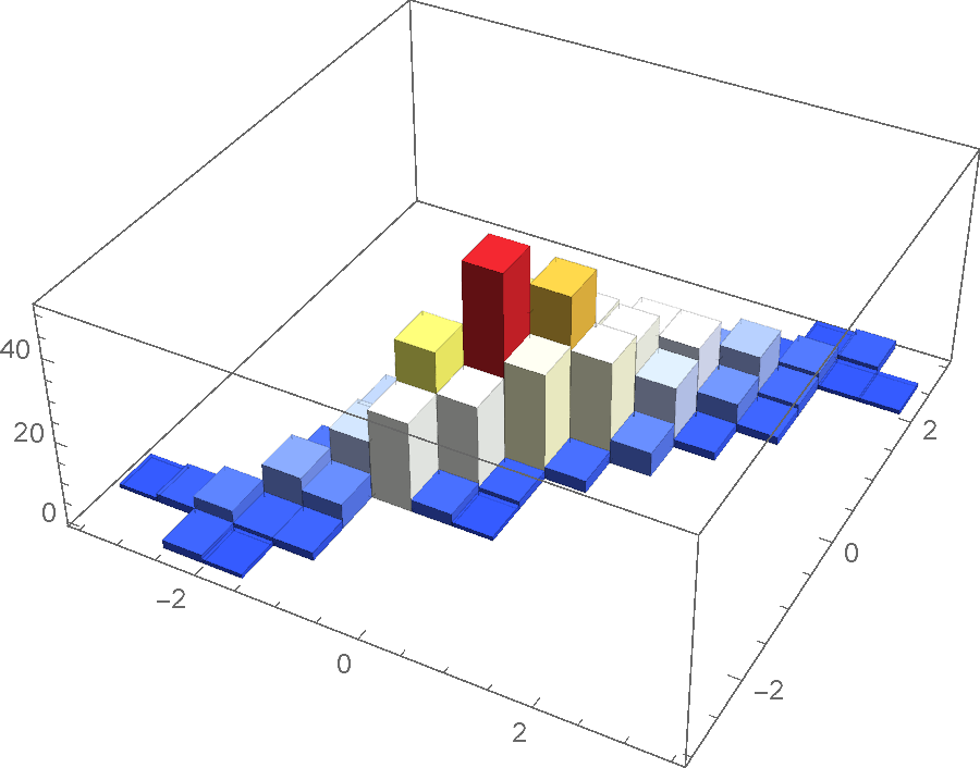
Here is some data sampled from a binormal distribution:
ClearAll["Global`*"];
pts = RandomVariate[BinormalDistribution[0.9], 500];
Histogram3D[pts, ColorFunction -> "TemperatureMap"]
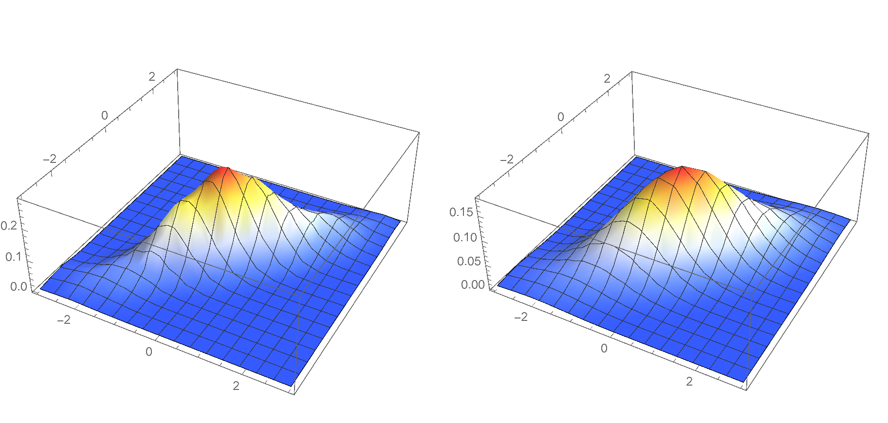
And here is the code that calculates the smooth kernel density estimate. The two plots are very similar; however, they are not entirely identical. Apparently, the SmoothKernelDensity[] calculation is more sophisticated. You may also follow this thread on Mathematica.SE for more information.
(* Use the built-in SmoothKernelDistribution[] *)
p1 = Plot3D[
  Evaluate@PDF[
    SmoothKernelDistribution[pts, MaxMixtureKernels -> All], {x, y}], {x, -3, 3}, {y, -3, 3},
    PlotRange -> All, ColorFunction -> "TemperatureMap"]

(* Manually calculate the smooth KDE *)
k[u_] := (1/(2 \[Pi])) * Exp[-u.u/2]
k[h_, u_] := Det[h]^(-1/2) * k[MatrixPower[h,-1/2].u]
f[x_, y_, h_] :=
 With[{n = Length@pts}, (1/n) *
    Sum[k[h, {x - First@pts[[i]], y - Last@pts[[i]]}], {i, 1, n}]] // N

h = SmoothKernelDistribution[pts]["Bandwidth"];
bw = {{First@h, 0}, {0, Last@h}};
p2 = Plot3D[f[x, y, bw], {x, -3, 3}, {y, -3, 3}, PlotRange -> All,
  ColorFunction -> "TemperatureMap"]

Style[Grid[{{p1, p2}}], ImageSizeMultipliers -> 1]