How to derive the Riemann curvature tensor
general relativity mathematics physics tensorsSo, I’ve decided to bite the bullet and study general relativity. I’ve been postponing it for quite a while, but the idea of my life ending without having studied one of the most profound and fundamental theories of physics was as much disturbing as motivating. I will be posting random stuff as I go and maybe I’ll come back later to edit them, as my understanding of the theory -hopefully- deepens.
I decided to watch the video lectures from Professor Susskind that are publicly available on YouTube. I liked them because Susskind puts an emphasis on the physical aspect of things and less on the formalism of the mathematics. Of course both are required, but for starters I think that it’s best to first build some intuition.
Our today’s goal is to come up with a tool to measure the curvature of space. Generally speaking, a change in the direction of a vector parallel-transported around a closed loop is a way to measure precisely this. Consider the following vector that is parallel-transported across \(A \rightarrow N \rightarrow B \rightarrow A\).
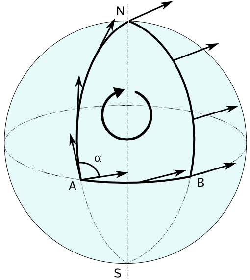
Image taken from here.
And notice how the initial vector and the final vector differ with an angle \(\alpha\). So, the idea is to compute the commutator of two covariant derivatives. This is as if we first move along the direction \(\mu\) and then \(\nu\) vs. first the direction \(\nu\) and then \(\mu\). Let us consider the action of this operator on a random vector \(V^\rho\):
\[\begin{align*} [\nabla_\mu, \nabla_\nu ] V^\rho &= \nabla_\mu \nabla_\nu V^\rho - \nabla_\nu \nabla_\mu V^\rho \\ &= \nabla_\mu \left[ \partial_\nu V^\rho + \Gamma_{\nu\sigma}^\rho V^\sigma \right] - (\mu \leftrightarrow \nu)\\ &= \partial_\mu \left[ \partial_\nu V^\rho + \Gamma_{\nu\sigma}^\rho V^\sigma \right] - \Gamma_{\mu \nu}^\lambda \left[ \partial_\lambda V^\rho + \Gamma_{\lambda \sigma}^\rho V^ \sigma\right] +\Gamma_{\mu\lambda}^\rho \left[ \partial_\nu V^\lambda + \Gamma_{\nu\sigma}^\lambda V^\sigma\right] - (\mu \leftrightarrow \nu)\\ &= \partial_\mu \partial_\nu V^\rho + \underbrace{\partial_\mu (\Gamma_{\nu\sigma}^\rho) V^\sigma + \Gamma_{\nu\sigma}^\rho \partial_\mu V^\sigma}_{\partial_\mu(\Gamma_{\nu\sigma}^\rho V^\sigma)} -\Gamma_{\mu\nu}^\lambda \partial_\lambda V^\rho - \Gamma_{\mu\nu}^\lambda \Gamma_{\lambda \sigma}^\rho V^\sigma + \Gamma_{\mu\lambda}^\rho \partial_\nu V^\lambda + \Gamma_{\mu\lambda}^\rho \Gamma_{\nu\sigma}^\lambda V^\sigma\\ &-\partial_\nu\partial_\mu V^\rho - \underbrace{\partial_\nu (\Gamma_{\mu\sigma}^\rho) V^\sigma - \Gamma_{\mu\sigma}^\rho \partial_\nu V^\sigma}_{\partial_\nu(\Gamma_{\mu\sigma}^\rho V^\sigma)} +\Gamma_{\nu\mu}^\lambda \partial_\lambda V^\rho + \Gamma_{\nu\mu}^\lambda \Gamma_{\lambda \sigma}^\rho V^\sigma - \Gamma_{\nu\lambda}^\rho \partial_\mu V^\lambda - \Gamma_{\nu\lambda}^\rho \Gamma_{\mu\sigma}^\lambda V^\sigma\\ &= \underbrace{\left[ \partial_\mu \Gamma_{\nu\sigma}^\rho - \partial_\nu \Gamma_{\mu\sigma}^\rho + \Gamma_{\mu\lambda}^\rho \Gamma_{\nu\sigma}^\lambda - \Gamma_{\nu\lambda}^\rho \Gamma_{\mu\sigma}^\lambda \right]}_{R_{\sigma\mu\nu}^\rho} V^\sigma\\ &= R_{\sigma\mu\nu}^\rho V^\sigma \end{align*}\]The directions \(\mu\) and \(\nu\) are our two transport directions, whereas \(\sigma\) is out initial direction. The tensor \(R_{\sigma\mu\nu}^\rho\) tells us the difference of the vectors obtained by transporting \(\partial\sigma\) first along \(\nu\) and then along \(\mu\) directions vs. the same vector obtained by first transporting along \(\mu\) and then \(\nu\). The index \(\rho\) is the \(\rho\)-th component.
Some useful tips for the above calculation:
- The covariant derivative of a type \((r,s)\) tensor field along \(\mu\) is given by the expression: \(\begin{align} {(\nabla_\mu T)^{a_1 \ldots a_r}}_{b_1 \ldots b_s} = {} &\frac{\partial}{\partial x^\mu}{T^{a_1 \ldots a_r}}_{b_1 \ldots b_s} \\ &+ \,{\Gamma ^{a_1}}_{\lambda\mu} {T^{\lambda a_2 \ldots a_r}}_{b_1 \ldots b_s} + \cdots + {\Gamma^{a_r}}_{\lambda\mu} {T^{a_1 \ldots a_{r-1}\lambda}}_{b_1 \ldots b_s} \\ &-\,{\Gamma^\lambda}_{b_1 \mu} {T^{a_1 \ldots a_r}}_{\lambda b_2 \ldots b_s} - \cdots - {\Gamma^\lambda}_{b_s \mu} {T^{a_1 \ldots a_r}}_{b_1 \ldots b_{s-1} \lambda}. \end{align}\)
Meaning that you take the ordinary partial derivative of the tensor and then add \(+{\Gamma^{a_i}}_{\lambda \mu}\) for every upper index \(a_i\) and \(-{\Gamma^\lambda}_{b_i \mu}\) for every lower index \(b_i\).
-
There are generalized Riemannian geometries that have torsion, in which the symmetry \(\Gamma_{\mu\nu}^\lambda = \Gamma_{\nu \mu}^\lambda\) does not hold. Those geometries are not widely used in ordinary gravitational theory. The geometry of general relativity is the Minkowski-Einstein geometry which is an extension of Riemannian geometry with a non-positive definite metric, but it doesn’t involve torsion.
-
Quantities that have different summation indices, but otherwise have the same symbols, are equal and cancel each other. For instance, \(\Gamma_{\mu\lambda}^\rho \partial_\nu V^\lambda\) is equal to \(\Gamma_{\mu\sigma}^\rho \partial_\nu V^\sigma\), because indices \(\lambda\) and \(\sigma\) are used just as dummy indices for the summation.
Example
Let us calculate the curvature of the surface of a sphere. To do that we need the Christoffel symbols \(\Gamma_{\mu\nu}^\lambda\) and since these symbols are expressed in terms of the partial derivatives of the metric tensor, we need to calculate the metric tensor \(g_{\mu\nu}\).
Calculation of metric tensor \(g_{\mu\nu}\)
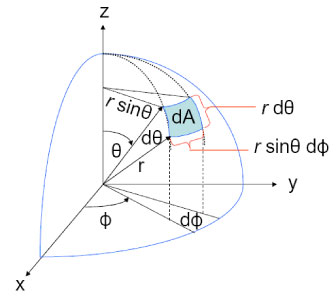
The following image illustrates the calculation of infinitestimal length \(\mathrm{d}S^2\) on the surface of a sphere.
But recall that:
\[\begin{align*} \mathrm{d}S^2 &= g_{\mu\nu} \mathop{\mathrm{d}x^\mu}\mathop{\mathrm{d}x^\nu } = \sum_{\mu=1}^2 \sum_{\nu=1}^2 g_{\mu\nu} \mathop{\mathrm{d}x^\mu}\mathop{\mathrm{d}x^\nu }\\ &= g_{11} \mathrm{d}x^1 \mathrm{d}x^1 + \underbrace{g_{12} \mathrm{d}x^1 \mathrm{d}x^2 + g_{21} \mathrm{d}x^2 \mathrm{d}x^1}_{\text{Equal due to symmetry}} + g_{22} \mathrm{d}x^2 \mathrm{d}x^2\\ &= g_{11} (\mathrm{d}x^1)^2 + 2g_{12} \mathrm{d}x^1 \mathrm{d}x^2 + g_{22} (\mathrm{d}x^2)^2 \end{align*}\]Let us use \(x^1 = \theta\) and \(x^2 = \phi\), then:
\[\begin{align*} dS^2 &= g_{\theta\theta} (\mathrm{d}\theta)^2 + 2g_{\theta\phi} \mathop{\mathrm{d}\theta} \mathop{\mathrm{d}\phi} &+ &g_{\phi\phi} (\mathrm{d}\phi)^2\\ &=R^2 \mathrm{d}\theta^2 &+ &R\sin^2\theta \mathrm{d}\phi^2 \end{align*}\]Therefore:
\[g_{\theta\theta} = R^2, g_{\theta\phi} = 0, g_{\phi\phi} = R\sin^2\theta\]And in matrix notation: \(\begin{pmatrix} g_{\theta \theta} & g_{\theta \phi} \\ g_{\phi \theta} & g_{\phi \phi} \end{pmatrix}= \begin{pmatrix} R^2 & 0 \\ 0 & R^2\sin^2\theta \end{pmatrix}\)
Calculation of the Christoffel symbols
Let us recall that the Christoffel symbol of the form \(\Gamma_{\mu\nu}^\lambda\) is given by the following formula:
\[\Gamma_{\mu\nu}^\lambda = \frac{1}{2}g^{\lambda\sigma} \left( \frac{\partial g_{\sigma\nu}}{\partial x^\mu} + \frac{\partial g_{\sigma\mu}}{\partial x^\nu} - \frac{\partial g_{\mu\nu}}{\partial x^\sigma}\right)= \frac{1}{2}g^{\lambda\sigma} \left( \partial_\mu g_{\sigma\nu} + \partial_\nu g_{\sigma\mu} - \partial_\sigma g_{\mu\nu}\right)\]At this point I’m going to cheat. Here is a function in Mathematica that calculates the \(\Gamma_{\mu\nu}^\lambda\):
ClearAll["Global`*"];
gmn = {{r^2, 0}, {0, r^2 Sin[\[Theta]]^2}};

InverseMetric[g_] := Simplify@Inverse@g

ChristoffelSymbol[g_, xx_] :=
 Block[{n, ig, res},
  n = 2;
  ig = InverseMetric[g];
  res = Table[
    (1/2) Sum[ig[[\[Lambda], \[Sigma]]]*
       (-D[g[[\[Mu], \[Nu]]], xx[[\[Sigma]]]] +
         D[g[[\[Sigma], \[Nu]]], xx[[\[Mu]]]] +
         D[g[[\[Sigma], \[Mu]]], xx[[\[Nu]]]]),
      {\[Sigma], 1, n}],
    {\[Lambda], 1, n}, {\[Mu], 1, n}, {\[Nu], 1, n}];
  Simplify[res]](*\[Lambda],\[Mu],\[Nu]*)

ChristoffelSymbol[gmn, {\[Theta], \[CurlyPhi]}][[1]]
(* {{0, 0}, {0, -Cos[\[Theta]] Sin[\[Theta]]}} *)

ChristoffelSymbol[gmn, {\[Theta], \[CurlyPhi]}][[2]]
(* {{0, Cot[\[Theta]]}, {Cot[\[Theta]], 0}} *)
Or a little prettier:
\[\Gamma_{\mu\nu}^\theta = \left( \begin{array}{cc} 0 & 0 \\ 0 & -\sin \theta \cos \theta \\ \end{array} \right)\qquad \Gamma_{\mu\nu}^\phi = \left( \begin{array}{cc} 0 & \cot \theta \\ \cot \theta & 0 \\ \end{array} \right)\]Let us remind ourselves of what the Christoffel symbol \(\Gamma_{\mu\nu}^\lambda\) means:
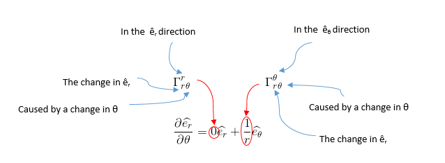
Image taken from here.
Now we are onto the calculation of the Riemann curvature tensor:
RiemannTensor[g_, xx_] :=
 Block[{n, Chr, res},
  n = 2;
  Chr = ChristoffelSymbol[g, xx];
  res = Table[
    D[Chr[[\[Rho], \[Nu], \[Sigma]]], xx[[\[Mu]]]] -
     D[Chr[[\[Rho], \[Mu], \[Sigma]]], xx[[\[Nu]]]] +
     Sum[Chr[[\[Rho], \[Mu], \[Lambda]]]*
       Chr[[\[Lambda], \[Nu], \[Sigma]]], {\[Lambda], 1, n}] -
     Sum[Chr[[\[Rho], \[Nu], \[Lambda]]]*
       Chr[[\[Lambda], \[Mu], \[Sigma]]], {\[Lambda], 1, n}],
    {\[Rho], 1, n}, {\[Sigma], 1, n}, {\[Mu], 1, n}, {\[Nu], 1, n}];
  Simplify[res]](*\[Rho],\[Sigma],\[Mu],\[Nu]*)
Let us calculate the component \(R_{\phi\theta\phi}^\theta\) for example.
RiemannTensor[gmn, {\[Theta], \[CurlyPhi]}]
(* {{{{0, 0}, {0, 0}}, {{0, Sin[\[Theta]]^2}, {-Sin[\[Theta]]^2,
    0}}}, {{{0, -1}, {1, 0}}, {{0, 0}, {0, 0}}}} *)
Or, in pretty format:
\[R = \left( \begin{array}{cc} \left( \begin{array}{cc} 0 & 0 \\ 0 & 0 \\ \end{array} \right) & \left( \begin{array}{cc} 0 & \sin^2 \theta \\ -\sin^2 \theta & 0 \\ \end{array} \right) \\ \left( \begin{array}{cc} 0 & -1 \\ 1 & 0 \\ \end{array} \right) & \left( \begin{array}{cc} 0 & 0 \\ 0 & 0 \\ \end{array} \right) \\ \end{array} \right)\]Therefore, \(R_{\phi\theta\phi}^\theta = \sin^2\theta\). Sometimes it’s more convenient to write the fully covariant version of the Riemann tensor (that is the tensor with all indices lowered), e.g.
\[\begin{align*} R_{\rho\sigma\mu\nu} &= g_{\rho \xi} R_{\sigma\mu\nu}^\xi \Rightarrow\\ R_{\theta\phi\theta\phi} &= g_{\theta \xi} R_{\phi\theta\phi}^\xi = \sum_{\xi=1}^2 g_{\theta \xi} R_{\phi\theta\phi}^\xi = g_{\theta \theta} R_{\phi\theta\phi}^\theta + g_{\theta \phi} R_{\phi\theta\phi}^\phi = R^2 \sin^2\theta \end{align*}\]since \(g_{\theta\theta} = R^2\) and \(g_{\theta\phi} = 0\).