The birthday paradox, factorial approximation and Laplace's method
Feynman integration integrals Laplace mathematics probabilitiesContents
- The birthday paradox
- Factorial \(n!\) approximation and the Stirling’s formula
- Laplace’s method for asymptotic integrals
The birthday paradox
So, I was looking at the birthday paradox and got a little carried away. Here’s how.
In probability theory, the birthday paradox or birthday problem refers to the probability that, in a set of \(N\) randomly chosen people, some pair of them will have birthday the same day. This probability reaches \(50\%\) with \(23\) people and \(99.9\%\) probability with just \(70\) people. It’s called a paradox because many people find these numbers too small and counter-intuitive.
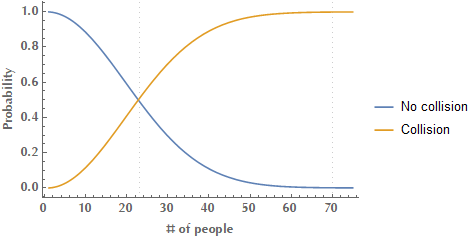
In order to calculate the probability of a birthday collision, it’s easier to start by considering the probability of “drawing” \(23\) people successively, so that each one has a birthday not yet seen. This is the probability of no collision, so the probability of at least one collision is its complementary, i.e. \(1\) minus this.
\[\begin{align*} \text{Prob}(\text{collision}) &= 1 - \text{Prob}(\text{No collision})\\ &= \underbrace{1 - \underbrace{\underbrace{\left(\frac{365}{365}\right)}_{\substack{\text{1st person has}\\\text{b-day not yet seen}}} \cdot \overbrace{\left(\frac{365-1}{365}\right)}^{\substack{\text{2nd person has}\\\text{b-day not yet seen}}} \cdot \left(\frac{365-2}{365}\right) \cdots \underbrace{\left(\frac{365-k+1}{365}\right)}_{\substack{k\text{-th person has}\\\text{b-day not yet seen}}}}_{\text{Probability of no collision}}}_{\text{Probability of collision}} \end{align*}\]Since it is:
\[\begin{align*} &\left(\frac{365}{365}\right) \cdot \left(\frac{365-1}{365}\right) \cdot \left(\frac{365-2}{365}\right) \cdots \left(\frac{365-k+1}{365}\right)\\ &=\frac{365 \cdot 364 \cdots (365-k+1)}{365^k}\\ &=\frac{365 \cdot 364 \cdots (365-k+1) \cdot (365-k) \cdot(365-k-1) \cdots 1}{365^k \cdot (365-k) \cdot(365-k-1) \cdots 1}\\ &= \frac{365!}{365^k (365-k)!}\\ &=\frac{365!/(365-k)!}{365^k} \end{align*}\]It follows that in a set of \(n\) randomly chosen items, the probability of some collision after \(k\) “draws” is:
\[\text{Prob(collision)} = 1 - \frac{n!/(n-k)!}{n^k}\]Factorial \(n!\) approximation and the Stirling’s formula
Since the calculation of birthday collision probability requires factorials of large numbers, naturally we would like to come up with a method to calculate them effortlessly. In this context, Stirling’s formula is an approximation for computing the factorial \(n!\). It is a decent approximation, giving accurate results even for small values of \(n\) and is named after James Stirling, a Scottish mathematician.
The formula that is usually referenced is the following:
\[\ln n! = n \ln{n} - n + \mathcal{O} (\ln n)\]In order to derive the above relation, we start with recognizing that:
\[n! = \int_0^\infty x^n e^{-x} \mathrm{d}x\]This is pretty straightforward to prove, just by applying repeatedly integration by parts. E.g.:
\[\begin{align*} I_1 &= -\int_0^\infty x^n \left(e^{-x}\right)' \mathrm{d}x = -\left[x^n e^{-x}\right]_0^\infty + \int_0^\infty n x^{n-1} e^{-x}\mathrm{d}x = n \int_0^\infty x^{n-1} e^{-x} \mathrm{d}x \end{align*}\]Similarly \(I_2 = n(n-1) \int_0^\infty x^{n-2} e^{-x} \mathrm{d}x\), and eventually the \(x^n\) will be exhausted and the factorial \(n!\) will have built up.
It turns out that there’s another method to do the calculation that is perhaps more slick and elegant. It was popularized by Richard Feynman, so it is often referred to as “Feynman integration”, although he did not invent it. The other name this method is known as is differentiation under the integral sign and it deserves a post on its own, but anyway. Here is how it goes for this particular case.
We define the following parameterized version of our integral:
\[g(k) = \int_0^\infty x^n e^{-k x} \mathrm{d}x\]We are interested in the value of \(g(1)\). As it will turn out, it’ll be easier to solve this more general problem and then set \(k=1\), than the original one! So:
\[\begin{align*} g(k) &= \frac{1}{(-1)^n} \int_0^\infty \frac{\mathrm{\partial}^n}{\mathrm{\partial} k^n} e^{-k x}\mathrm{d}x = \frac{1}{(-1)^n} \frac{\mathrm{d}^n}{\mathrm{d}k^n} \int_0^\infty e^{-k x}\mathrm{d}x = \frac{1}{(-1)^n} \frac{\mathrm{d}^n}{\mathrm{d}k^n} \left( \left.\frac{e^{-k x}}{-k}\right|_0^\infty \right)\\ &= \frac{1}{(-1)^n} \frac{\mathrm{d}^n}{\mathrm{d}k^n} \left( \frac{1}{k} \right) = \frac{1}{(-1)^n} (-1)^n \frac{n!}{k^{n+1}} = \frac{n!}{k^{n+1}} \end{align*}\]Finally:
\[g(1) = \int_0^\infty x^n e^{-x} \mathrm{d} x = \frac{n!}{1^{n+1}} = n!\]So as long as we can approximate the value of the above integral, we can approximate the value of \(n!\). Well, let us summon Pierre-Simon, marquis de Laplace.
Laplace’s method for asymptotic integrals
The Laplace’s method enables us to approximate the value of the following integral as \(\lambda \to \infty\):
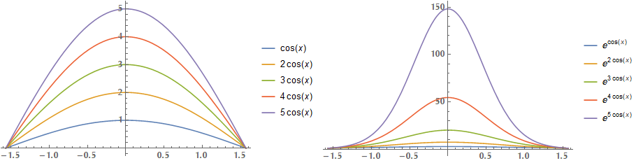
\[I(\lambda) = \int_a^b f(x) e^{-\lambda \varphi(x)} \mathrm{d}x\]The idea behind this method is that the value of the integral is dominated by the values of \(e^{-\lambda \varphi(x)}\) around the minimum point of \(\varphi(x)\) (therefore, around the maximum point of \(-\lambda \varphi(x)\). Here you can see the effect of raising \(\lambda \cos{x}\) in \(e\). In specific, you can see how the exponentiation makes the function to approximate a Gaussian function and how the value of the integral is dominated by a small region around the maximum point of \(\lambda \cos{x}\), in specific around \(x_0 = 0\).
Our assumptions include the convergence of \(I(\lambda)\) for sufficiently large \(\lambda\), that \(f(x)\) and \(\varphi(x)\) are smooth enough to be replaced by their local Taylor expansions of appropriate degree. Also \(\varphi'(x_0) = 0, \varphi''(x_0) > 0\) (therefore \(\varphi(x_0)\) is a minimum and \(-\lambda \varphi(x_0)\) a maximum) and \(f(x_0)\ne0\).
We linearize \(f(x)\) and expand \(\varphi(x)\) into a second order Taylor series around the point \(x=x_0\):
\[\begin{align*} f(x) \simeq f(x_0), \qquad \varphi(x) &\simeq \varphi(x_0) + \underbrace{\varphi'(x_0) (x-x_0)}_{\text{zero, since } \varphi'(x_0)=0} + \frac{1}{2}\varphi''(x_0) (x-x_0)^2 + \ldots\\ &= \varphi(x_0) + \frac{1}{2}\varphi''(x_0) (x-x_0)^2 + \ldots \end{align*}\]Therefore:
\[\begin{align*} I(\lambda) &\simeq f(x_0) \int_a^b \exp\left[ -\lambda \left(\varphi(x_0) + \frac{1}{2}\varphi''(x_0)(x-x_0)^2\right)\right] \mathrm{d}x\\ &= f(x_0) e^{-\lambda \varphi(x_0)} \int_a^b e^{-\frac{\lambda}{2}\varphi''(x_0)(x-x_0)^2} \mathrm{d}x\\ &= f(x_0) e^{-\lambda \varphi(x_0)}\int_a^b e^{-\frac{\lambda}{2}\varphi''(x_0)s^2} \mathrm{d}s \end{align*}\]Recall that for Gaussian integral it is:
\[\int_{-\infty}^{+\infty} e^{-a x^2} \mathrm{d}x = \sqrt{\frac{\pi}{a}}\]Here it is \(\frac{\lambda}{2}\varphi''(x_0) = a\), therefore:
\[\begin{align*} I(\lambda) &\simeq f(x_0) e^{-\lambda \varphi(x_0)} \sqrt{\frac{\pi}{\frac{\lambda}{2}\varphi''(x_0)}}\\ &= f(x_0) e^{-\lambda \varphi(x_0)} \sqrt{\frac{2\pi}{\lambda \varphi''(x_0)}} \end{align*}\]Laplace’s method for deriving Stirling’s approximation
Alright, so the idea is to bring the integral \(I(n) = \int_0^\infty x^n e^{-x}\mathrm{d}x\) to the form \(I(n) = \int_0^\infty f(x) e^{-n \varphi(x)}\mathrm{d}x\), because we already have a formula for the latter. So
\[I(n) = \int_0^\infty x^n e^{-x}\mathrm{d}x = \int_0^\infty e^{\ln x^n} e^{-x}\mathrm{d}x = \int_0^\infty e^{n \ln x} e^{-x}\mathrm{d}x = \int_0^\infty e^{n \ln x -x}\mathrm{d}x\]We are close, but not quite yet. If only we could write \(x\) as a multiple of \(n\), then we could factor out \(n\) and be done. Therefore, let’s try to substitute \(x = n z \Rightarrow \mathrm{d}x = n \mathrm{d}z\):
\[I(n) = n\int_0^\infty e^{n \ln (n z) - n z}\mathrm{d}z = n\int_0^\infty e^{n \ln n} e^{n \ln z - n z}\mathrm{d}z = n^{n+1} \int_0^\infty e^{-n \overbrace{\left(z - \ln{z}\right)}^{\varphi(z)}}\mathrm{d}z\]Yes! We are exactly where we would like to be since \(f(z) = 1, \varphi(z) = z - \ln{z}\) and \(\varphi'(z) = 1 - 1/z \Rightarrow z_0 = 1, \varphi'(z_0) = 0\) and \(\varphi''(z) = 1/z^2 \Rightarrow \varphi''(z_0) = 1\).
Finally:
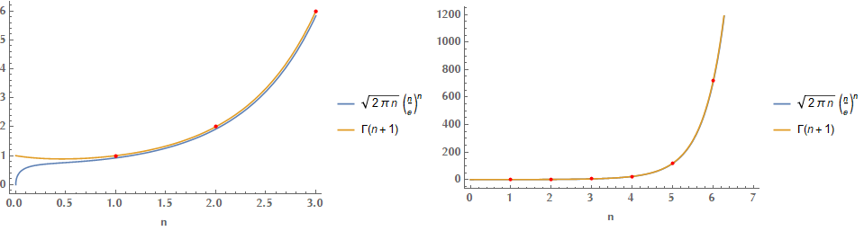
\[\begin{align*} n! &\simeq n^{n+1} f(z_0) e^{-n \varphi(z_0)} \sqrt{\frac{2\pi}{n \varphi''(z_0)}}\\ &= n^{n+1} e^{-n} \sqrt{\frac{2\pi}{n}}\\ &= \sqrt{2\pi} n^{n+1/2} e^{-n} \end{align*}\]
Another example of Laplace’s method
Suppose we would like to calculate the value of the following integral:
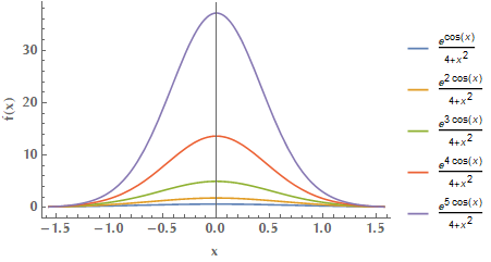
\[I(\lambda) = \int_0^{\pi/2} \frac{e^{\lambda \cos x}}{x^2+4} \mathrm{d}x = \frac{1}{2} \int_{-\pi/2}^{\pi/2} \frac{e^{-\lambda \overbrace{(-\cos x)}^{\varphi(x)} }}{x^2+4} \mathrm{d}x\]Since the function we integrate is symmetric, i.e. \(g(x) = g(-x)\) it follows that \(\int_{-a}^{a} g(x)\mathrm{d} x = 2 \int_0^a g(x) \mathrm{d}x\). Why did we change the interval of integration from \([0, \pi/2]\) to \([-\pi/2, \pi/2]\)? Well, because we want \(\varphi(x)\) to have a local minimum in the interior of the interval upon which we integrate.
Therefore:
\[I(\lambda) = f(x_0) e^{-\lambda \varphi(x_0)} \sqrt{\frac{2\pi}{\lambda \varphi''(x_0)}}\]In our case \(f(x) = \frac{1}{x^2+4}\) and \(\varphi(x) = -\cos x\). It is \(\varphi'(x) = \sin x \Rightarrow x_0 = 0\) and \(\varphi''(x_0) = \cos x_0 = 1 > 0\). So
\[I(\lambda) = \frac{1}{2} \frac{1}{x_0^2 + 4} e^{-\lambda (-\cos x_0)} \sqrt{\frac{2\pi}{\lambda \cos x_0}} = \sqrt{\frac{\pi}{32\lambda}} e^{\lambda}\]Here is the function we integrated for increasing values of \(\lambda\):