Common misconceptions about exponential growth
covid-19 exponential medicineCoronavirus disease 2019 (COVID-19) is an infectious disease caused by Severe Acute Respiratory Syndrome CoronaVirus 2 (SARS-CoV-2). At the time of writing Covid-19 has become a global pandemic. In many countries where lockdown was not enforced early on, coronavirus cases showed an exponential growth. After having talked to many people the last days, I came to understand that there are some common misconceptions regarding how an exponential function behaves. Here are my thoughts on this matter.
Misconception 1: Lack of fast growth, rules out exponential dynamics.
Many people think that exponential increase is a synonym for explosive, fast, immense growth. This may be true eventually, but for “small” values of \(x\), an exponential function can be, initially, approximated by a linear function. This means that an exponential growth may masquerade as a linear function during the early phase of the phenomenon.
Why is that? Recall how \(\exp(x)\) can be expressed as a Maclaurin series:
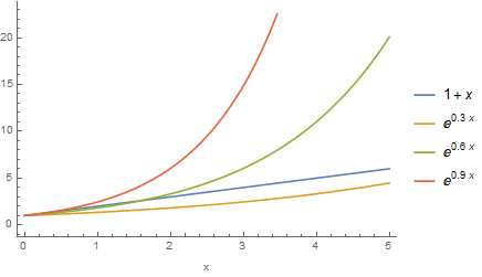
\[\exp(x) = 1 + x + \frac{1}{2}x^2 + \frac{1}{6}x^3 + \ldots\]For “small” values of \(x\), the contributions of higher order terms (those containing \(x^2\), \(x^3\), …) are minuscule. Therefore, in this case, the approximation \(\exp(x) \simeq 1 + x\) holds. Similarly, if we take a look at \(\exp(\lambda x)\), where the constant \(\lambda\) tunes the growth rate, its Maclaurin series is:
\[\exp(\lambda x) = 1 + \lambda x + \underbrace{\frac{1}{2}\lambda^2 x^2 + \frac{1}{6}\lambda^3 x^3 + \ldots}_{\text{Negligible for } \lambda\ll 1\text{ and small } x }\]Depending on the value of \(\lambda\), the exponential function may trick us, for an extended period of time, into thinking that it’s linear. In the following image you may see how for different values of \(\lambda < 1\), the respective functions hide their exponential nature for longer time (for larger values of \(x\)).
Another example of an exponential change, that may span a very large amount of time, is the radioactive decay of Uranium-238. U-238 is the most common isotope of uranium found in nature and has a half-life of ~4.5 billion years. This means that the quantity of U-238 you have, will be reduced to its half after ~4.5 billion years. The mathematical formula describing this physical process is given by:
\[N(t) = N_0 \exp(-\lambda t)\]Where \(t\) is the elapsed time, \(N_0\) is the initial quantity of the radioactive material (the material at \(t=0\)), \(\lambda\) is the decay parameter (affecting how fast or slow the process is) and \(N(t)\) is the quantity after time \(t\) has elapsed. For U-238 the decay constant \(\lambda\) is approximately equal to \(1.54 \times 10^{-10} \text{year}^{-1}\).
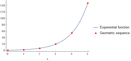
Misconception 2: Exponential is “faster” than geometric
The difference between an exponential function and a geometric sequence is that the first takes continuous values, whereas the latter discrete. It doesn’t have anything to do with the rate of change.
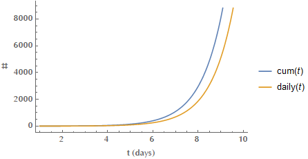
Misconception 3: The cumulative number of cases may be exponential, but the daily number of cases need not be exponential.
Let us assume that the cumulative number of cases up until time \(t\) is given by the exponential formula: \(\text{cum}(t) = \exp(t)\). Then, the number of daily cases at time \(t\) can be calculated via the following logic:
\[\begin{align*} \text{cum}(t) = \exp(t) \Rightarrow \text{daily}(t) &= \text{cum}(t)-\text{cum}(t-1)\\ &= \exp(t) - \exp(t-1)\\ &= e^t \left(1 - \frac{1}{e}\right) = a e^t \end{align*}\]So, the number of daily new cases is given by an exponential form as well. You can’t have exponentially increasing cumulative number of cases, without having exponential daily new cases.