Normality tests in statistics
mathematics R language statisticsContents
Introduction
Some statistical tests (e.g., t-test for independent samples or ANOVA) assume that the data in question are modeled by a normal distribution. Therefore, before using such a test, one must first confirm that the data do not deviate much from normality. There are many ways to do this, and ideally, one should combine them. These include looking at the mean/median (should be approximately equal), skewness (should be approximately zero), kurtosis (should be around three), histograms (should be approximately bell-shaped), Q-Q plots (should roughly form a line) and, ultimately, running a normality test, such as Shapiro-Wilk.
A typical example
So, suppose we are given a dataset with sodium excretion values of some male and female individuals. We’d like to perform, say, a t-test to see whether their means differ significantly. First, we need to check whether our data follow a normal distribution.
Descriptive statistics
We start by printing some summary descriptive statistics:
df %>%
  group_by(gender) %>%
  summarize(
    n = n(),
    min = min(sodium.excretion, na.rm = TRUE),
    q1 = quantile(sodium.excretion, 0.25, na.rm = TRUE),
    median = quantile(sodium.excretion, 0.5, na.rm = TRUE),
    q3 = quantile(sodium.excretion, 0.75, na.rm = TRUE),
    max = max(sodium.excretion, na.rm = TRUE),
    mean = mean(sodium.excretion, na.rm = TRUE),
    sd = sd(sodium.excretion, na.rm = TRUE),
    skewness = skewness(sodium.excretion, na.rm = TRUE),
    kurtosis = kurtosis(sodium.excretion, excess = FALSE, na.rm = TRUE))

# A tibble: 2 x 11
  gender     n   min    q1 median    q3   max  mean    sd skewness kurtosis
  <chr>  <int> <dbl> <dbl>  <dbl> <dbl> <dbl> <dbl> <dbl>    <dbl>    <dbl>
1 F         26   0.2  131.   157.  172.  242.  139.  58.1  -1.23       4.29
2 M         26  95.9  136.   152.  174.  201.  157.  26.6   0.0430     2.70
>
Notice that for males (M), the median and mean are close to each other (subjectively), whereas, for females (F), the difference is considerable. Also, skewness is close to zero for M’s and smaller than -1 for F’s. Last, the kurtosis for M’s is approximately equal to 3, as ought to be for the distribution to be normal. On the contrary, kurtosis in F’s dataset is well beyond 3. Considering these, we hypothesize that M’s sodium excretion values are sampled from a normal distribution, whereas F’s values are not.
Visualisation
We proceed by taking a look at the data:
df %>%
    ggplot(aes(x = sodium.excretion, fill = gender)) +
    geom_density(alpha = 0.5) + facet_wrap(~ gender) +
    theme_bw() +
    labs(x = "Sodium excretion (mmol/day)", y = "Density",
         title = "Sodium excretion",
         subtitle = "By gender", fill = "Group")
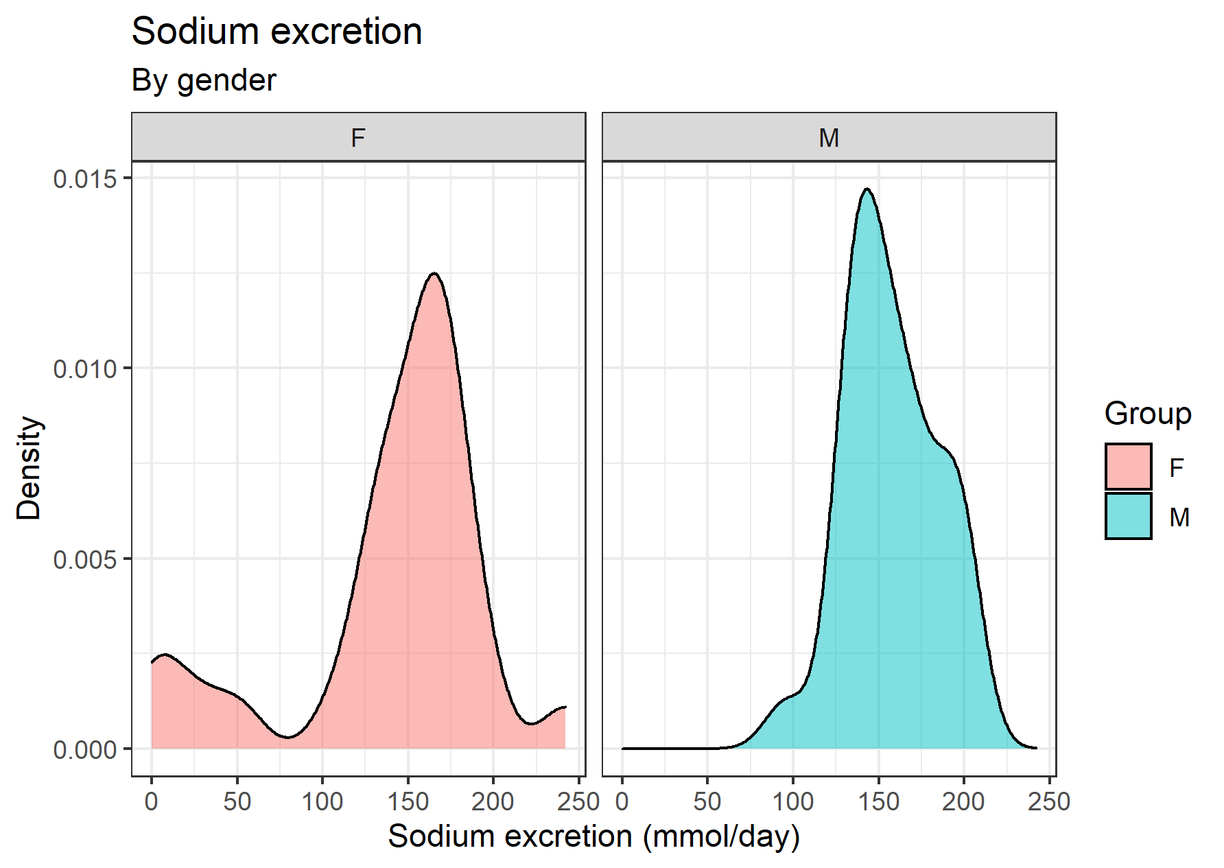
The curve of sodium excretion in male individuals is what you’d expect for an histogram of small sample size, more or less. The curve of the females, though, has some fat tail at the left. That’s a hint that perhaps it deviates from normality. Let’s take a look at the Q-Q plots broken down by the gender factor variable:
df %>%
  ggplot(aes(sample = sodium.excretion, col = gender)) +
  stat_qq() + stat_qq_line() +
  labs(x = "Theoretical Quantiles", y = "Sample Quantiles", col = "Gender") +
  theme_bw()
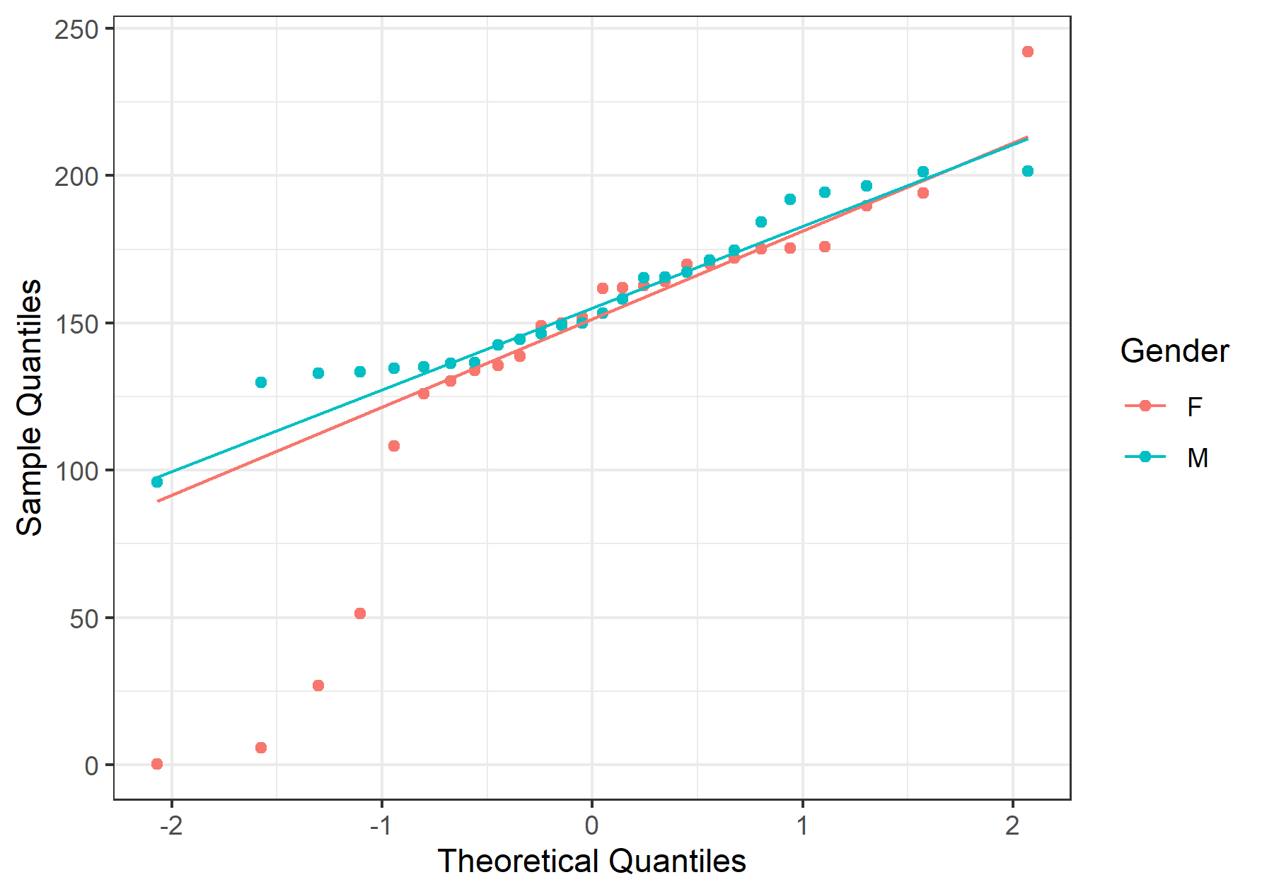
Consistent with whatever has been seen so far, the male Q-Q plot’s data points fall onto a straight line. On the other hand, in females, the data points deviate a lot at the tail. Again, this builds upon the hypothesis that M’s distribution is normal, and F’s is not.
Shapiro-Wilk test
The final step is to actually run a normality test, such as Shapiro-Wilk’s:
df %>%
  group_by(gender) %>%
  shapiro_test(sodium.excretion)

# A tibble: 2 x 4
  gender variable         statistic       p
  <fct>  <chr>                <dbl>   <dbl>
1 F      sodium.excretion     0.847 0.00123
2 M      sodium.excretion     0.947 0.200
>
The results are consonant with our previous findings. The p-value of the Shapiro-Wilk test in the females group is \(p = 0.00123\), whereas for the males is \(p = 0.2\). Therefore, assuming a confidence level \(a = 0.05\), we reject the null hypothesis for the females (i.e., we reject that data are normally distributed) and accept it for the males’ group (i.e., we accept that data are normally distributed). This was a pretty straightforward example, given that all the results of our exploratory analysis agreed with each other.
But what happens when, for example, plots and Shapiro-Wilk test disagree?
Disagreement between plots and Shapiro-Wilk test
What happens when the plots say that the data aren’t normally distributed, but the Shapiro-Wilk test disagrees? Or vice versa?
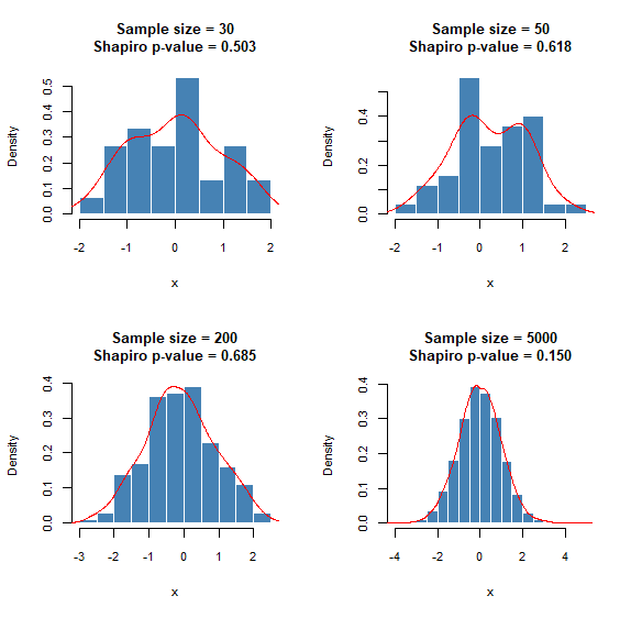
For small sample sizes, the histograms rarely resemble the shape of a normal distribution, and that’s fine. As soon as one increases the sample size, the shape of the distribution converges to that of the underlying distribution. On the other hand, the Shapiro-Wilk test correctly implies normality, as you can see in the p-values of the following plot.
Here is the R code that generates the above plots:
################################################################################
# NORMAL DISTRIBUTION
################################################################################
plot_sample <- function(sample_size) {
sample_dist <- rnorm(sample_size, mean = 0, sd = 1)
sp <- shapiro.test(sample_dist)
par(ps = 10)
hist(sample_dist, xlab = "x",
main = sprintf("Sample size = %d\nShapiro p-value = %.3f",
sample_size, sp$p.value),
col = "steelblue", border = "white", prob = T)
lines(density(sample_dist), col = "red")
}
par(mfrow = c(2, 2))
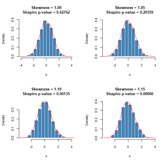
lapply(c(30, 50, 200, 5000), plot_sample)Shapiro-Wilk test begins to behave in a “problematic” manner when the sample size is large. In the following plots, I’ve fixed the sample size equal to 5000 (this is the largest allowed value for R’s shapiro.test() anyway). Notice how the test rejects normality even for slightly skewed normal distributions. On the other hand, histograms look pretty good! To be fair, the Shapiro-Wilk test isn’t at fault here. It’s just that it does its job so well, by detecting even tiny deviations from normality, that it no longer serves our purpose: to detect large deviations from a normal distribution.
And the R code:
################################################################################
#                             SKEWED NORMAL DISTRIBUTION
################################################################################
library(fGarch)

plot_sample2 <- function(skewness_param) {
    N <- 5000
    sample_dist <- rsnorm(n = N, mean = 0, sd = 1, xi = skewness_param)
    sp <- shapiro.test(sample_dist)
    par(ps = 10)
    hist(sample_dist, xlab = "x",
        main = sprintf("Skewness = %.2f\nShapiro p-value = %.5f",
                       skewness_param, sp$p.value),
        col = "steelblue", border = "white", prob = T)
    lines(density(sample_dist), col = "red")
}
par(mfrow = c(2, 2))
lapply(c(1, 1.05, 1.1, 1.15), plot_sample2)
Conclusion
So, the rule of thumb I follow is this: if histograms and Shapiro-Wilk disagree, for a small sample size, I go with Shapiro-Wilk. For a large sample size, I go with the histograms. Of course, either way, I take into consideration the descriptives and Q-Q plots. And one more thing! For many tests, it doesn’t really matter whether your data are normally distributed, as long as your samples’ mean follows the normal distribution. However, this is fulfilled by the central limit theorem, assuming your samples are sufficiently large. This is the subject of another post!