Benford's law and COVID-19 conspiracy theories
covid-19 mathematics R language statisticsContents
Introduction
How can we know if a list of numbers is made up or has come up in a “natural” way?
This question may sound distant at first, but it has several applications. In the 2016 film, “The Accountant”, Ben Affleck’s character uses Benford’s law, which we’ll talk about today, to expose fraud in a robotics company. In particular, he notes that the digit “3” appears more often than expected in some financial numerical data.

Benford’s law, also called the law of “irregular numbers” or law of “the first digit”, is an observation about how often different numbers appear as digits in real numbers. The law states that in many cases (but not all!) when we have lists of numbers produced by a natural process (e.g., number of coronavirus infections 😉), the most significant digit is likely to be small.
The number “1” appears as the most significant digit in about 30% of cases, while “9” appears in less than 5% of cases. If the digits were evenly distributed, we would encounter each with a frequency of about 11.1% (f=1/9 * 100%). The law also makes predictions for the distribution of second digits, third digits, combinations of digits, etc.
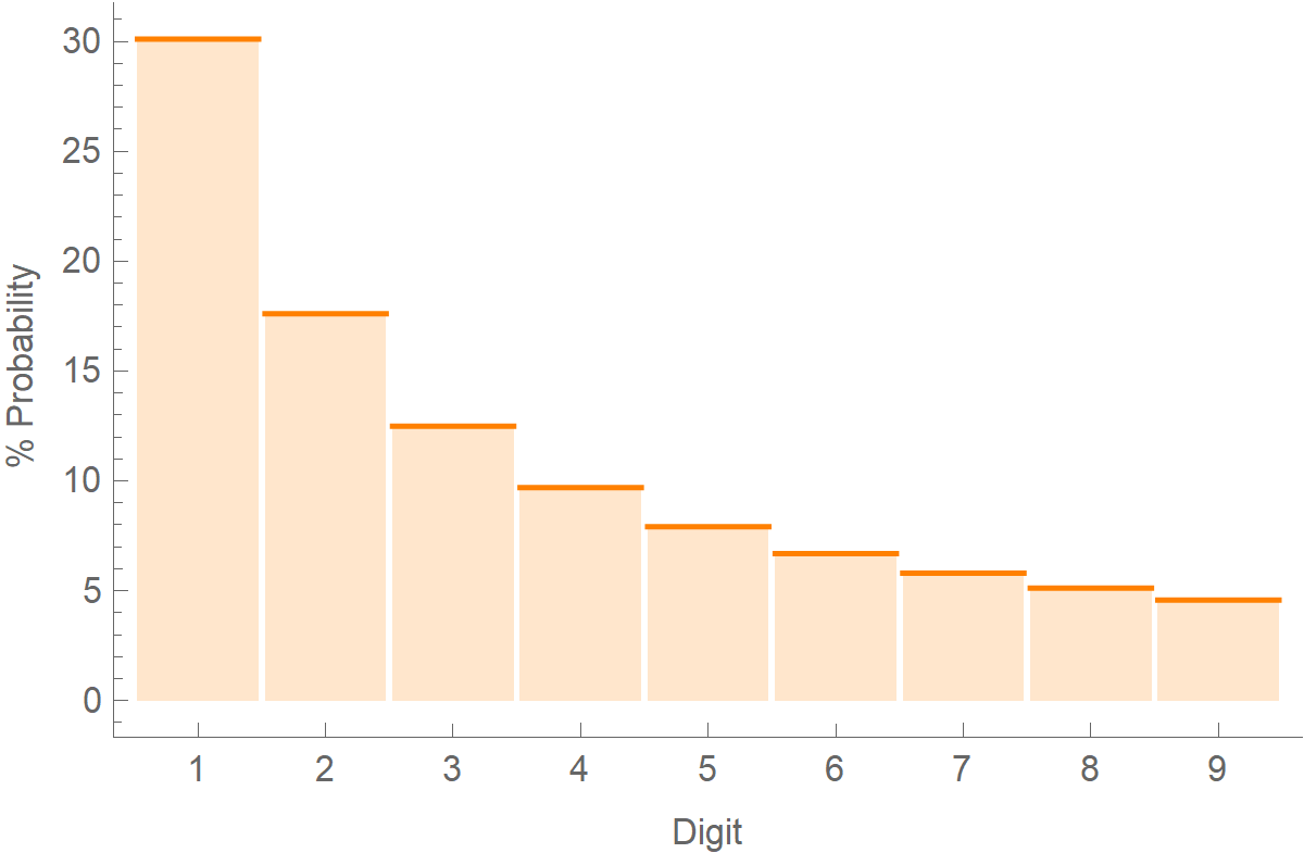
The formula for calculating the probabilities of various digits is this:
\[\text{Prob}(d) = \text{log}_{10} \left( 1 + \frac{1}{d}\right)\]When making up numbers, people who are unaware of Benford’s law tend to distribute their digits evenly. Thus, a mere comparison of the first or second digit frequency distribution could easily show “abnormal” results.
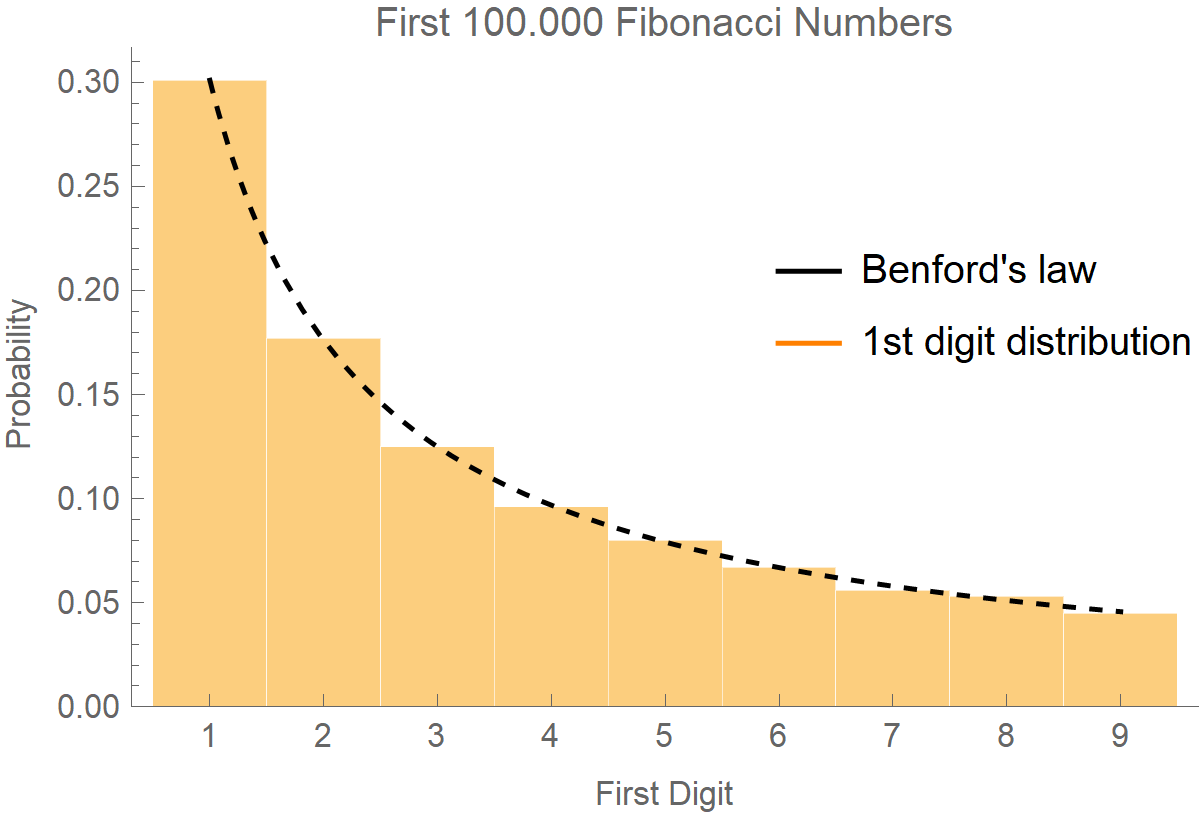
It’s amazing how many numerical distributions follow this law, like the Fibonacci numbers:
Legended[
 Show[
  Histogram[
   First /@ IntegerDigits /@ Table[Fibonacci[k], {k, 1, 100000}],
   Automatic, "PDF",
   Frame -> {True, True, False, False},
   FrameLabel -> {"First Digit", "Probability"},
   FrameTicks -> {Range[1, 9], Automatic},
   PlotLabel -> "First 100.000 Fibonacci Numbers",
   ChartBaseStyle -> EdgeForm[White]],
  Plot[Log10[1 + 1/d], {d, 1, 9}, PlotStyle -> {Black, Dashed}]],
 Placed[LineLegend[{Black, Orange}, {"Benford's law", "1st digit distribution"}], {.8, .6}]]
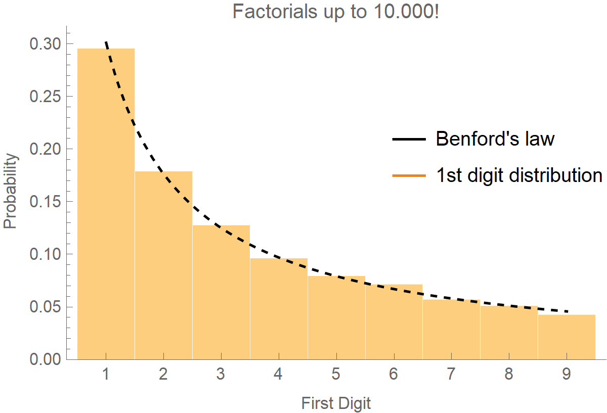
Or, the factorials:
Legended[
 Show[
  Histogram[
   First /@ IntegerDigits /@ Table[Factorial[k], {k, 1, 10000}],
   Automatic, "PDF",
   Frame -> {True, True, False, False},
   FrameLabel -> {"First Digit", "Probability"},
   FrameTicks -> {Range[1, 9], Automatic},
   PlotLabel -> "Factorials up to 10.000!",
   ChartBaseStyle -> EdgeForm[White]],
  Plot[Log10[1 + 1/d], {d, 1, 9}, PlotStyle -> {Black, Dashed}]],
 Placed[LineLegend[{Black, Orange}, {"Benford's law", "1st digit distribution"}], {.8, .6}]]
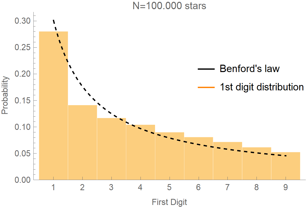
Or, the distances of stars from Earth:
starsData = EntityValue["Star", "DistanceFromEarth"];
Legended[
 Show[
  Histogram[
   First /@ First /@ RealDigits /@
      Select[
       QuantityMagnitude /@
        UnitConvert[Take[stardat, 100000], "meters"],
       NumberQ],
   Automatic, "PDF", Frame -> {True, True, False, False},
   FrameLabel -> {"First Digit", "Probability"},
   FrameTicks -> {Range[1, 9], Automatic},
   PlotLabel -> "N=100.000 stars", ChartBaseStyle -> EdgeForm[White]],
  Plot[Log10[1 + 1/d], {d, 1, 9}, PlotStyle -> {Black, Dashed}]],
 Placed[LineLegend[{Black, Orange}, {"Benford's law", "1st digit distribution"}], {.8, .6}]]
Benford’s law on COVID-19 data
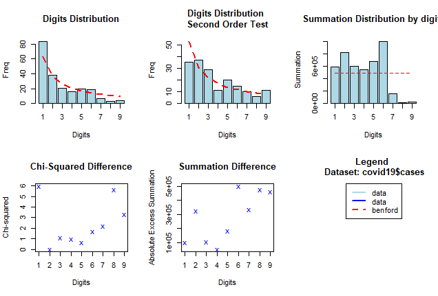
In the figure below, we have plotted how often the various digits appear in the number of coronavirus cases of the USA’s Washington state. We got the data from this link, and we can not guarantee their authenticity. However, it appears that the distribution of numbers in the 1st and 2nd most significant position of the number of cases approaches the theoretical distribution of Benford’s law (dotted red line), so we can not assume that someone “cooked” the data, within the confidence interval, the statistics provide.
library(benford.analysis)
us <- read_csv("C:\\Users\\stathis\\Downloads\\us-states.csv")
covid19 <- us[us$state == "Washington",]
bfd.cp <- benford(covid19$cases, number.of.digits = 1)
plot(bfd.cp)
In this article the authors performed a thorough analysis and found that records of cumulative infections and deaths from the United States, Japan, Indonesia and most European nations adhered well to the Benford’s law, consistent with accurate reporting. Their results can be found here.
Benford’s law on SIR data
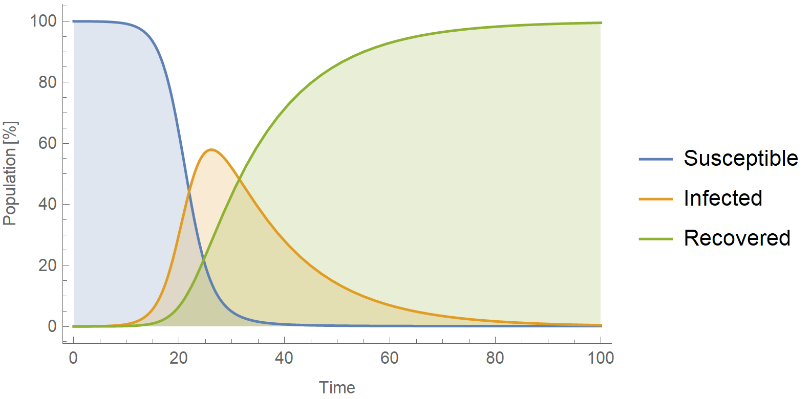
For the fun of it, the following Mathematica code solves a simple SIR model and draws the frequency distribution of the first digit in the number of infected people. In short a SIR model is described by the following set of differential equations:
\[\left\{ \frac{\mathrm{d}S}{\mathrm{d}t}=-\beta S I, \hspace{0.75cm}\frac{\mathrm{d}I}{\mathrm{d}t}=\beta S I - \gamma I, \hspace{0.75cm}\frac{\mathrm{d}R}{\mathrm{d}t}=\gamma I \right\}\]Where \(t\) is the time, \(S\) is the number of susceptible people, \(I\) is the number of people infected, and \(R\) is the number of people who have recovered and developed immunity to the infection (thus they are no longer susceptible to re-infection). The parameter \(\beta\) is the infection rate, and \(\gamma\) is the recovery rate.
ClearAll["Global`*"];

eqS = s'[t] == -b*s[t]*i[t];
eqI = i'[t] == b*s[t]*i[t] - gamma*i[t];
eqR = r'[t] == gamma*i[t];

b = 0.5; gamma = 1/14.0;

solution =
  NDSolve[
   {eqS, eqI, eqR, s[0] == 1, i[0] == 0.0001, r[0] == 0}, {s, i, r}, {t, 1000}];

solS = s /. solution[[1, 1]];
solI = i /. solution[[1, 2]];
solR = r /. solution[[1, 3]];

Plot[{100*solS[t], 100*solI[t], 100*solR[t]}, {t, 0, 100},
 PlotLegends -> {"Susceptible", "Infected", "Recovered"},
 Frame -> {True, True, False, False}, FrameLabel -> {"Time", "Population [%]"}, Filling -> Bottom]
This is the evolution of the SIR model:
And this is the frequency distribution of the first digits superimposed with the theoretical Benford’s distribution (dotted black line):
numbers = Table[solI[t], {t, 0, 200}];
digits = RealDigits /@ numbers;

p1 = ListPlot[
   Table[PDF[BenfordDistribution[10], x], {x, 1, 9}],
   Joined -> True, PlotRange -> All, PlotStyle -> {Red, Dashed}];

Show[
 Histogram[
  digits[[All, 1, 1]], Automatic, "PDF",
  Frame -> {True, True, False, False}, FrameLabel -> {"Digits", "Probability"},
  FrameTicks -> {Range[1, 9], Automatic}, PlotTheme -> "Monochrome"],
 p1]
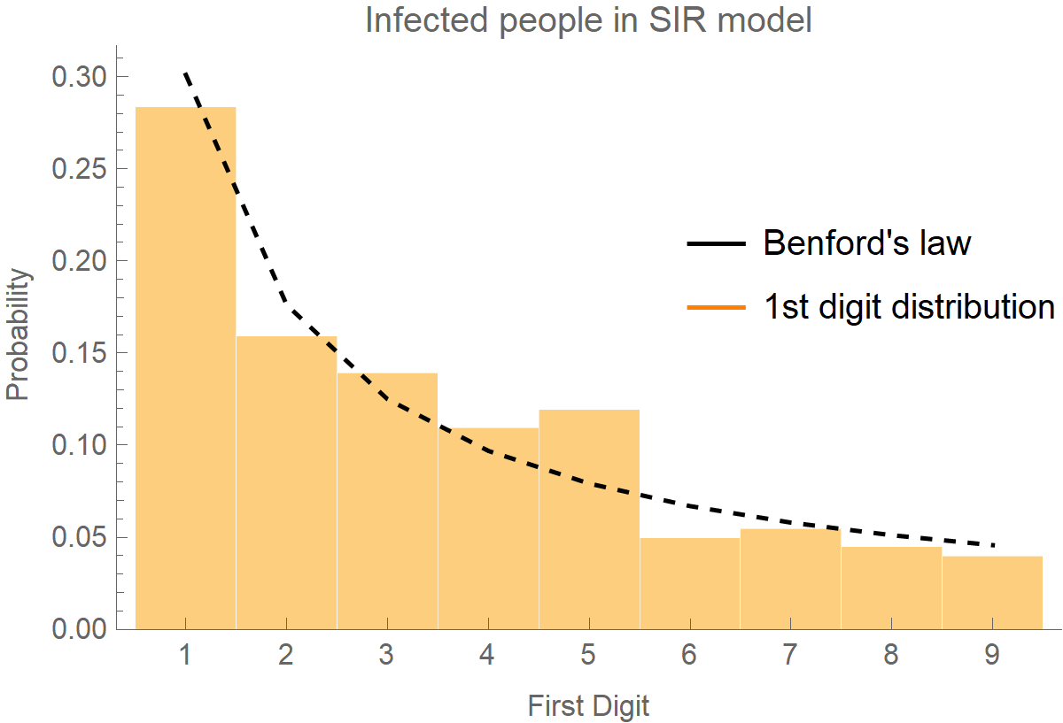
By the way, if you plot the frequency distribution of the first digits for the recovered cases, the data do not follow Benford’s law.
Relevant work
If you are interested in the topic of verifying COVID-19 epidemiological data, you should really check the following paper by the team of Nicholas Christakis: Jia, J. S. et al. Population flow drives spatio-temporal distribution of COVID-19 in China. Nature 582, 389–394 (2020). In this work, the researchers used geolocation data from mobile phones in China to generate collective population movements from Wuhan to the mainland. It turned out, that people’s geographical flow was on par with the subsequent outbreaks in the rest of mainland China as far as location, intensity, and timing were concerned! Besides verification, though, what’s more important regarding this modeling is the following. By looking at how people move during an epidemic, we may be able to forecast where the epidemic will strike in the next weeks and take measures to mitigate it. How awesome science is?