Principal component analysis with Lagrange multiplier
Lagrange multiplier machine learning mathematics optimization Principal Component Analysis statisticsContents
The motivation
It is often the case that we are given a dataset with many variables to analyze. One of the widely used methods is to seek linearly correlated variables in the dataset. Once we have identified these variables, we replace them with new ones, called principal components, that are linear combinations of the original variables.
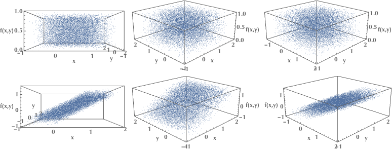
In the first row of the following plots, we examine a set of data points that span the whole 3D space uniformly. Since there are no correlations between the \(x,y,z\) variables, we could not possibly compress our description of the dataset and get away using only two variables. However, in the second row, we see a set of points lying, more or less, on a plane. In this case, we could use just two variables and still locate them in the 3D space with decent accuracy. The intrinsic dimension of our data is the 2D plane, not the 3D space.
This transformation of data from a high-dimensional space into a low-dimensional one, which preserves some essential qualities of the original data, is called dimensionality reduction. Working with fewer dimensions has many advantages, such as being able to create visualizations in 2 or 3 dimensions that humans are comfortable to work with.
The formulation
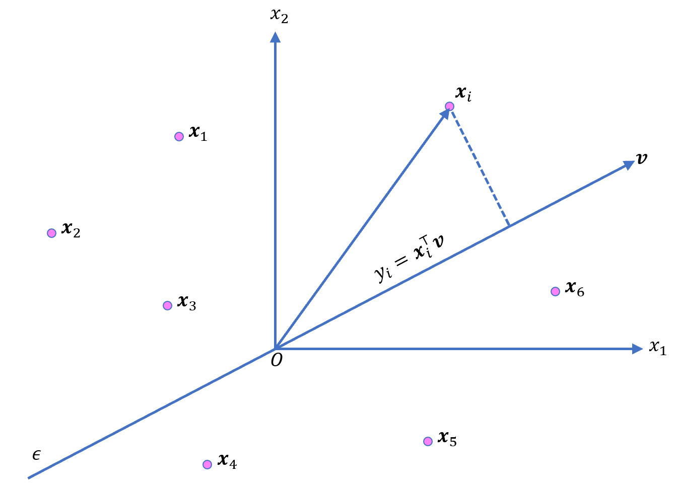
Suppose that we have \(\mathbf{x}_1,\mathbf{x}_2,…,\mathbf{x}_n\) centered points in \(m\) dimensional space. Let \(\mathbf{v}\) denote the unit vector along which we project our \(\mathbf{x}\)’s. The length of the projection \(y_i\) of \(\mathbf{x}_i\) is \(y_i = \mathbf{x}_i^⊤ \mathbf{v}\).
The mean squared projections summed over all points \(\mathbf{x}_i\) is the variance \(V\):
\[\begin{align*} V &= \frac{1}{n} \sum_{i=1}^n y_i^2 = \frac{1}{n}\sum_{i=1}^n\left(\mathbf{x}_i^⊤ \mathbf{v}\right)^2\\ &=\frac{1}{n}\sum_{i=1} \mathbf{x}_i^⊤ \mathbf{v} \cdot\mathbf{x}_i^⊤ \mathbf{v} = \frac{1}{n}\sum_{i=1} \mathbf{v}^⊤ \mathbf{x}_i \cdot\mathbf{x}_i^⊤ \mathbf{v}\\ &= \mathbf{v}^⊤ \underbrace{\left(\frac{1}{n}\sum_{i=1}^n \mathbf{x}_i \mathbf{x}_i^⊤\right)}_{\text{Covariance matrix}}\mathbf{v} = \mathbf{v}^⊤ C \mathbf{v} \end{align*}\]Mind that the covariance matrix is defined as:
\[C = \frac{1}{n} \sum_{i=1}^n \left(\mathbf{x}_i - \mu\right)\left(\mathbf{x}_i -\mu\right)^⊤\]Where \(\mu\) is the mean of \(\mathbf{x}_i, i = 1,2,\ldots,n\). Which is why we asked for the variables \(\mathbf{x}_i\) to be centered. So that \(\mu=0\) and the formula for covariance would simplify to \(C = \frac{1}{n} \sum_{i=1}^n \mathbf{x}_i \mathbf{x}_i^⊤\).
Our objective is to maximize variance \(V\) subject to the constraint \(\|\mathbf{v}\|=1\). Such problems of constrained optimization might be reformulated as unconstrained optimization problems via the use of Lagrangian multipliers. If we’d like to maximize \(f(\mathbf{x})\) subject to \(g(\mathbf{x})=c\), we introduce the Lagrange multiplier \(\lambda\) and construct the Lagrangian \(\mathcal{L}(\mathbf{x},\lambda)\):
\[\mathcal{L}(\mathbf{x},\lambda) = f(\mathbf{x}) - \lambda(g(\mathbf{x})-c)\]The sign of \(\lambda\) doesn’t make any difference. We then solve the system of equations:
\[\left\{\frac{\partial\mathcal{L} (\mathbf{x}, \lambda)}{\partial \mathbf{x}} = 0, \, \frac{\partial \mathcal{L}(\mathbf{x}, \lambda)}{\partial \lambda} = 0\right\}\]The solution
In our case, we want to maximize Variance \(V\) subject to the constraint \(\|\mathbf{v}\|=1 \Leftrightarrow \mathbf{v}^⊤\mathbf{v} = 1\). Our Lagrangian is:
\[\mathcal{L}(\mathbf{v},\lambda) = \mathbf{v}^⊤ C \mathbf{v} - \lambda(\mathbf{v}^⊤ \mathbf{v}-1)\]We solve for the stationary points:
\[\begin{align*} \frac{\partial \mathcal{L}}{\partial \mathbf{v}} &= 2\mathbf{v}^⊤ \mathbf{C} - 2\lambda \mathbf{v}^⊤ = 0\\ \frac{\partial \mathcal{L}}{\partial \lambda} &= \mathbf{v}^⊤ \mathbf{v} - 1 = 0 \end{align*}\]And we end up with the following eigenvector equation:
\[C \mathbf{v} = \lambda \mathbf{v}\]Note: In case you don’t recall it, as I did not, the derivative of quadratic form \(\mathbf{x}^⊤ \mathbf{A} \mathbf{x}\) with respect to vector \(\mathbf{x}\) is \(\mathbf{x}^⊤(\mathbf{A} + \mathbf{A}^⊤)\). And since the covariance matrix \(C\) is symmetric, i.e. \(\mathbf{C}=\mathbf{C}^⊤\), it follows that:
\[\frac{\partial}{\partial\mathbf{v}} \left( \mathbf{v}^⊤ \mathbf{C} \mathbf{v}\right) = \mathbf{v}^⊤\left(\mathbf{C} + \mathbf{C}^⊤\right)=2\mathbf{v}^⊤\mathbf{C}\]Example with one principal component
Strong linear correlation case
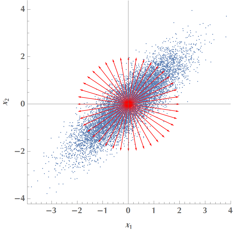
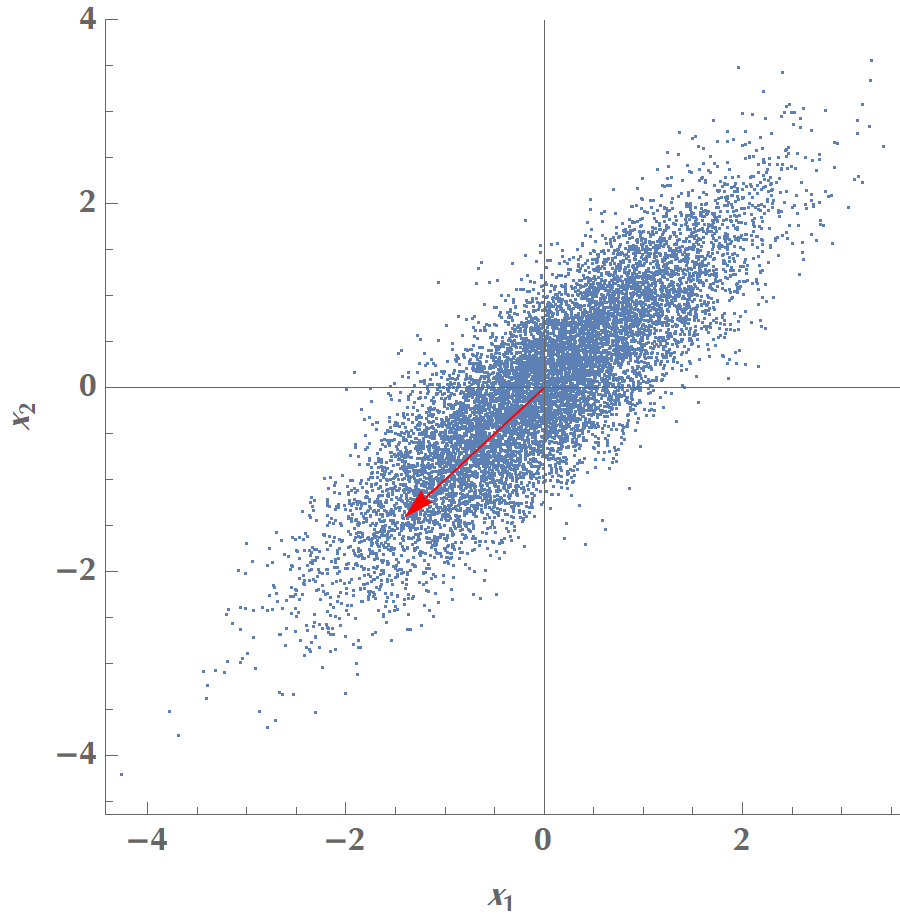
Let us play with the simplest possible scenario, where we have two variables, \(x_1\) and \(x_2\), and we’d like to calculate a single principal component. In the graph below, we plot the data along with various candidate vectors \(\mathbf{v}\) pointing in different directions. Our goal is to find the one vector \(\mathbf{v}\), which will maximize the data points’ variance when projected on the line the vector defines.
If we plot the variance as a function of angle of \(\mathbf{v}\) with the \(x\) axis, we get the following:
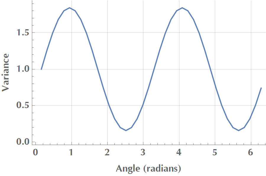
In the image above, we see that \(V\) reaches a maximum when the vector aligns with the data’s elongated axis. Then it is reduced until it reaches a minimum when the vector orientates vertically to the elongated axis. In total, two vectors maximize variance, and they are opposite to each other, but the sign of \(\mathbf{v}\) doesn’t really matter.
You could play with the following code to reproduce the experiment:
ClearAll["Global`*"];
(*Create some random points from a bivariate normal distribution*)
npts = 10000;
pts = RandomVariate[BinormalDistribution[{0, 0}, {1, 1}, 0.85], npts];
var[v_] := (1/npts) Sum[(pts[[i]].v)^2, {i, npts}]
angleStep = Pi/20.;
vs = Table[{Cos[theta], Sin[theta]}, {theta, 0, 2 Pi, angleStep}];
varvs = var /@ vs;
maxpos = Ordering[varvs, -1][[1]];
vs[[maxpos]]
(*{-0.707107,-0.707107}*)
You could also solve the eigenvector equation \(C\mathbf{v} = \lambda\mathbf{v}\):
Eigenvectors[Covariance[pts]][[1]]
(* {0.707107, 0.707107} *)
Weak linear correlation
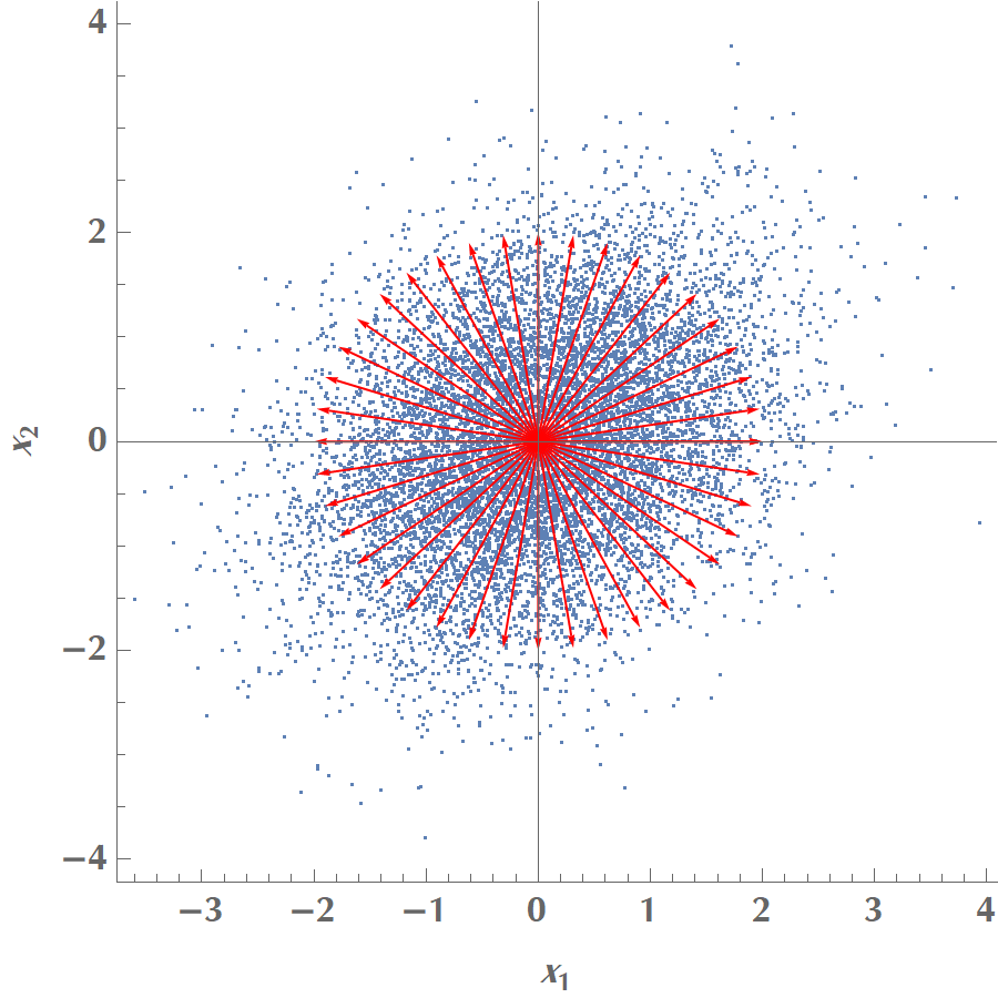
Let us now repeat the experiment, but this time \(x_1\) and \(x_2\) will have a weak linear correlation. Same as before, we draw many vectors along different orientations:
We then calculate the variance of our projected data onto the various vectors and plot the results as a function of angle:
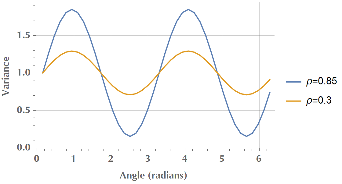
In the image above, we see that \(V\)’s amplitude was reduced when we transitioned from variables with strong correlation (\(\rho = 0.85\)) to variables with weak correlation (\(\rho = 0.3\)). It’s getting clear that as \(x_1\) and \(x_2\) become less (linearly) correlated, we have a hard time to find a unique direction in space along which variance is maximized. In the limit where \(\rho = 0\), any direction would do! That’s why, before applying PCA, we usually test for the existence of linear correlations in our dataset, via scatterplots, correlation matrix or Bartlett’s test of sphericity.