Custom training loops and subclassing with Tensorflow

Contents

• Introduction
• Fit linear regression model to data by minimizing MSE
  • Generate training data
  • Create a custom Keras layer
  • Define a custom loss function
  • Train the model with a custom training loop
• Fit Gaussian curve to data with maximum likelihood estimation
  • What is likelihood?
  • A concrete example of maximum likelihood estimation
  • How is mean squared error related to log-likelihood?

Introduction

The most straightforward way to train a model in Tensorflow is to use the model.fit() and model.fit_generator() Keras functions. These functions may seem opaque at first, but they accept callbacks that make them versatile. Such callbacks enable early stopping, saving the model to the disk periodically, writing logs for TensorBoard after every batch, accumulating statistics, and so on. However, it may be the case that one needs even finer control of the training loop. In this post, we will see a couple of examples on how to construct a custom training loop, define a custom loss function, have Tensorflow automatically compute the gradients of the loss function with respect to the trainable parameters, and then update the model.

Fit linear regression model to data by minimizing MSE

Generate training data

The “Hello World” of data science is arguably fitting a linear regression model. Indeed, in the first example, we will first generate some noisy data, and then we will fit a linear regression model of the form \(y = m x + b\). The model’s parameters are the scalars \(m, b\), and their optimal values will be figured out by Tensorflow.

import tensorflow as tf
tf.__version__

# '2.4.0'

import matplotlib
import matplotlib.pyplot as plt
import numpy as np

def generate_noisy_data(m, b, n=100):
    """ Generates (x, y) points along the line y = m * x + b
    and adds some gaussian noise in the y coordinates.
    """
    x = tf.random.uniform(shape=(n,))
    noise = tf.random.normal(shape=(len(x),), stddev=0.15)
    y = m * x + b + noise
    return x, y

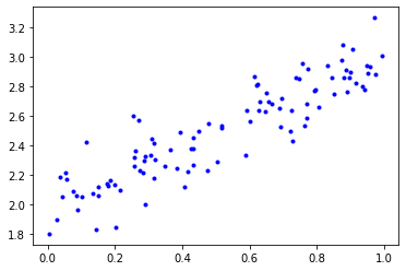
x_train, y_train = generate_noisy_data(m=1, b=2)
plt.plot(x_train, y_train, 'b.');

Create a custom Keras layer

We then subclass the tf.keras.layers.Layer class to create a new layer. The new layer accepts as input a one dimensional tensor of \(x\)’s and outputs a one dimensional tensor of \(y\)’s, after mapping the input to \(m x + b\). This layer’s trainable parameters are \(m, b\), which are initialized to random values drawn from the normal distribution and to zeros, respectively.

class LinearRegressionLayer(tf.keras.layers.Layer):
    def __init__(self):
        super(LinearRegressionLayer, self).__init__()
        self.m = self.add_weight(shape=(1,), initializer='random_normal')
        self.b = self.add_weight(shape=(1,), initializer='zeros')

    def call(self, inputs):
        return self.m * inputs + self.b

# Instantiate a LinearRegressionLayer and call it on our x_train tensor
linear_regression_layer = LinearRegressionLayer()
linear_regression_layer(x_train)

#    <tf.Tensor: shape=(100,), dtype=float32, numpy=
#    array([6.32419065e-03, 1.72153376e-02, 6.32639334e-04, 5.57286246e-03,
#           1.25469696e-02, 1.44133652e-02, 9.44772546e-05, 1.12606948e-02,
#           5.26433578e-03, 1.16873141e-02, 1.17568867e-02, 1.61101166e-02,
#           4.66661761e-03, 1.65831670e-02, 1.31081808e-02, 5.73157147e-03,
#           ...
#           5.68887964e-03, 1.30544147e-02, 1.70514826e-02, 9.80825396e-04],
#          dtype=float32)>

Define a custom loss function

Here, we define our custom loss function. For this particular case, the mean squared error (MSE) is appropriate, but conceivably we could use whatever loss function we’d like.

def MSE(y_pred, y_true):
    """Calculates the Mean Squared Error between y_pred and y_true vectors"""
    return tf.reduce_mean(tf.square(y_pred - y_true))

We calculate our loss function for the newly instantiated linear regression layer. At the moment, the parameters \(m\) have random values and \(b=0\), so we expect MSE to be high.

# Calculate the MSE for the initial m, b values
MSE(linear_regression_layer(x_train), y_train)

#    <tf.Tensor: shape=(), dtype=float32, numpy=6.283869>

Train the model with a custom training loop

Here comes the custom training loop. What is essential in the following code is the tf.GradientTape[] context. Every operation that is performed on the input inside this context is recorded by Tensorflow. We will then use this record for automatic differentiation.

# Custom training loop
learning_rate = 0.05
epochs = 30

mse_loss = []
for i in range(epochs):
    with tf.GradientTape() as tape:
        predictions = linear_regression_layer(x_train)
        current_mse_loss = MSE(predictions, y_train)

    gradients = tape.gradient(current_mse_loss, linear_regression_layer.trainable_variables)
    linear_regression_layer.m.assign_sub(learning_rate * gradients[0])
    linear_regression_layer.b.assign_sub(learning_rate * gradients[1])
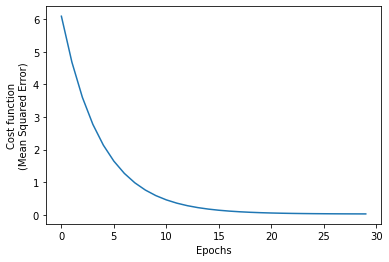
    mse_loss.append(current_mse_loss)

We confirm that the algorithm converged by looking at the MSE vs. epoch:

plt.plot(mse_loss)
plt.xlabel('Epochs')
plt.ylabel('Cost function\n(Mean Squared Error)');

We print the optimal values for the models’ parameters, \(m, b\), after the training has completed. Indeed, \(m_\text{opt} = 1.05, b_\text{opt} = 1.91\) are very close to the ground truth values (minus the noise we added).

# Print optimal values for the parameters m, b.
# The ground truth values are m = 1, b = 2.
linear_regression_layer.m, linear_regression_layer.b

#    (<tf.Variable 'Variable:0' shape=(1,) dtype=float32, numpy=array([1.053719], dtype=float32)>,
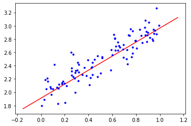
#     <tf.Variable 'Variable:0' shape=(1,) dtype=float32, numpy=array([1.911512], dtype=float32)>)

Finally, we superimpose the training data with the best linear regression model Tensorflow converged to:

# Generate evenly spaced numbers over the initial x interval plus some margin
x = np.linspace(min(min(x_train), -0.15), max(max(x_train), 1.15), 50)

# Plot the optimal y = m * x + b regression line superimposed with the data
plt.plot(x, linear_regression_layer.m * x + linear_regression_layer.b, 'r')
plt.plot(x_train, y_train, 'b.');

Fit Gaussian curve to data with maximum likelihood estimation

What is likelihood?

Likelihood measures how well a statistical model fits a sample of data given a set of values for the unknown parameters. It is considered a function of the parameters only, treating the random variables as fixed at their observed values.

For instance, suppose that we are given a sample \(x_1, x_2, \ldots, x_N\) and we are told that the underlying distribution is normal, but the model’s parameters, \(\mu, \sigma^2\), are unknown to us. How could we estimate those parameters? We start by considering the probability density function (PDF) of the normal distribution:

\[f(x\mid \mu, \sigma^2) = \frac{1}{\sqrt{2\pi\sigma^2} } \exp\left(-\frac {(x-\mu)^2}{2\sigma^2} \right)\]

Then, we define as likelihood \(\mathcal{L}\) the corresponding PDF for the whole sample (assuming independent identically distributed) of normal random variables:

\[\mathcal{L}(\mu,\sigma^2 \mid x_1,\ldots,x_N) = \prod_{i=1}^N f(x_i) = \left( \frac{1}{\sqrt{2\pi\sigma^2}} \right)^{N} \exp\left( -\frac{ \sum_{i=1}^N (x_i-\mu)^2}{2\sigma^2}\right)\]

Notice how we treat \(\mathcal{L}(\mu,\sigma^2 \mid x_1,\ldots,x_N)\) as a function of the model’s parameters \(\mu, \sigma^2\), and the \(x_i\) as fixed. Therefore, given a set of observations and a candidate model parameterized by some parameters (here \(\mu,\sigma^2\)), likelihood measures how well the model accounts for the observation of these data.

A more concrete example is this. Suppose we observe just three values: 0.5, 2, and 1. Assuming the underlying distributions is Gaussian, what would then be \(\mathcal{L}\) equal to?

\[\mathcal{L}(\mu,\sigma ^2\mid x=0.5, 2, 1) = \frac{1}{\sqrt{2 \pi \sigma^2}} e^{-\frac{(0.5 -\mu)^2}{2 \sigma^2}}\times \frac{1}{\sqrt{2 \pi \sigma^2}} e^{-\frac{(2 -\mu)^2}{2 \sigma^2}}\times \frac{1}{\sqrt{2 \pi \sigma^2}} e^{-\frac{(1 -\mu)^2}{2 \sigma^2}}\]

Now that we have a formula for \(\mathcal{L}\), we can plug in different values of \(\mu, \sigma^2\) and calculate the likelihood. The combination of \(\mu,\sigma^2\) that yields the largest likelihood will constitute our best estimate. By the way, it’s easier to work with logarithms every time we deal with a product, and this is how the log-likelihood concept emerges:

\[\begin{align*} \log \mathcal{L}(\mu,\sigma^2 \mid x_1,\ldots,x_N) &= \log \prod_{i=1}^N f(x_i) \\ &=\log\left[\left( \frac{1}{\sqrt{2\pi\sigma^2}} \right)^{N} \exp\left( -\frac{ \sum_{i=1}^N (x_i-\mu)^2}{2\sigma^2}\right)\right]\\ &=-\frac{N}{2} \log \left( 2\pi \sigma^2 \right) - \sum_{i=1}^{N} \left( \frac{(x_i - \mu)^2}{2\sigma^2}\right) \end{align*}\]

Ok, let’s do some experimentation with Python now:

def pdf(x, m, s):
    """Returns the probability that x was sampled from a normal
    distribution with mean m and standard deviation s."""
    return (1/(2 * np.pi * s**2)**0.5) * math.exp(-0.5 * ((x - m)/s)**2)

# Generate some random normally distributed numbers
dat = np.random.normal(0, 1, 5)
for x in dat:
    print("Probability of x = {:6.3f} coming from a N(0,1) distribution = {:6.2f}%".
          format(x, 100 * pdf(x, 0, 1)))

# Probability of x =  1.295 coming from a N(0,1) distribution =   6.88%
# Probability of x = -1.276 coming from a N(0,1) distribution =   7.05%
# Probability of x = -0.084 coming from a N(0,1) distribution =  15.86%
# Probability of x =  0.830 coming from a N(0,1) distribution =  11.28%
# Probability of x = -0.920 coming from a N(0,1) distribution =  10.42%

At this point we have considered every observation on its own. Now we will view the sample as a whole and calculate the joint PDF of all \(x_i\):

# Probability that all numbers were randomly drawn from a normal distribution with m = 0, s = 1
np.prod( [pdf(x, 0, 1) for x in dat] )

# 9.043067752419683e-06

# Probability that all numbers were randomly drawn from a normal distribution with m = 2, s = 1
np.prod( [pdf(x, 2, 1) for x in dat] )

# 3.0081558180762395e-10

Since it’s easier to work with logarithms every time we deal with a product, as we are in this case, we take the log of the likelihood:

# Log-likelihood that all numbers were randomly drawn from a normal distribution with m = 0, s = 1
math.log( np.prod( [pdf(x, 0, 1) for x in dat] ) )

# -11.613512087983674

# Log-likelihood that all numbers were randomly drawn from a normal distribution with m = 2, s = 1
math.log( np.prod( [pdf(x, 2, 1) for x in dat] ) )

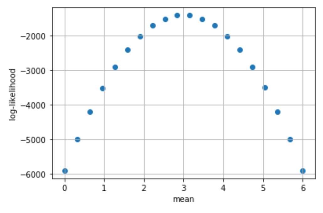
# -21.924523723972346

Our ultimate goal is to find the optimal values for the model’s parameters, \(\mu, \sigma^2\), that maximize the log-likelihood. If they maximize the log-likelihood, they will also maximize the likelihood. However, it’s typical for an optimizer to minimize a cost function by default rather than maximize a utility function. Therefore, we usually define our cost function to be the negative log-likelihood, and have our optimizer minimize it. By minimizing the negative log-likelihood, we maximize the log-likelihood (and therefore the likelihood).

# Generate 1000 normally distributed numbers with mean = 3, std = 1
dat = np.random.normal(3, 1, 1000)

# Try a range of possible mean values and calculate the
# log-likelihood. For brevity, we fix std to be 1.
mus = np.linspace(0, 6, 20)
ll = []
for m in mus:
    # log(a * b * c ...) = log(a) + log(b) + log(c) + ...
    current_ll = np.sum([math.log(pdf(x, m, 1)) for x in dat])
    ll.append([m, current_ll])
    
x, y = zip(*ll)
plt.scatter(x, y)
plt.xlabel('mean')
plt.ylabel('log-likelihood')
plt.grid(True)

A concrete example of maximum likelihood estimation

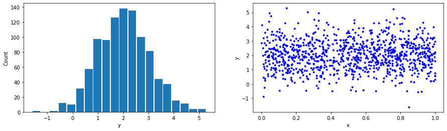
In the second example, we will generate some data sampled from a normal distribution with known parameters. We will then use Tensorflow to figure out the optimal model’s parameters that maximize our data’s negative log-likelihood.

def generate_gaussian_data(m, s, n=1000):
    x = tf.random.uniform(shape=(n,))
    y = tf.random.normal(shape=(len(x),), mean=m, stddev=s)
    return x, y

# Generate normally distributed data with mean = 2 and std dev = 1
x_train, y_train = generate_gaussian_data(m=2, s=1)

plt.figure(figsize=(15, 4))
plt.subplot(1, 2, 1)
plt.hist(y_train, bins=20, rwidth=0.9)
plt.xlabel('y')
plt.ylabel('Count')

plt.subplot(1, 2, 2)
plt.plot(x_train, y_train, 'b.')
plt.xlabel('x')
plt.ylabel('y');

The same as before, we subclass the tf.keras.layers.Layer and add our model’s parameters as weights. We initialize their values to whatever value the user supplies. We then instantiate a new layer with some estimated values for the parameters that are purposely off.

class GaussianFitLayer(tf.keras.layers.Layer):
    def __init__(self, ivs):
        super(GaussianFitLayer, self).__init__()
        self.m = self.add_weight(shape=(1,), initializer=tf.keras.initializers.Constant(ivs[0]))
        self.s = self.add_weight(shape=(1,), initializer=tf.keras.initializers.Constant(ivs[1]))

    def call(self, inputs):
        y = tf.random.normal(shape=(len(inputs),), mean=self.m, stddev=self.s)
        return y

# Come up with some initial values (they are off on purpose),
# so that we can check whether the optimization algorithm converges.
m0 = 0.7 * tf.reduce_mean(y_train)
s0 = 1.3 * tf.math.reduce_std(y_train)
gaussian_fit_layer = GaussianFitLayer([m0, s0])

We then define a function that calculates the negative log-likelihood, given some observed values and a set of parameters.

def nll(y_true, params):
    """Calculates the Negative Log-Likelihood for a given set of parameters"""
    N = len(y_true)
    m, s = params
    return (N/2.) * tf.math.log(2. * np.pi * s**2) + (1./(2.*s**2)) * tf.math.reduce_sum((y_true - m)**2)

Here comes the custom training loop. The code is almost identical to the previous case. It’s just the loss function that differs.

# Custom training loop
learning_rate = 0.0005
epochs = 50

nll_loss = []
for i in range(epochs):
    with tf.GradientTape() as tape:
        current_nll_loss = nll(y_train, [gaussian_fit_layer.m, gaussian_fit_layer.s])
    gradients = tape.gradient(current_nll_loss, gaussian_fit_layer.trainable_variables)
    gaussian_fit_layer.m.assign_sub(learning_rate * gradients[0])
    gaussian_fit_layer.s.assign_sub(learning_rate * gradients[1])
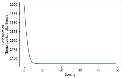
    nll_loss.append(current_nll_loss)

We confirm that the algorithm converged, and also we print the best estimates for the model’s parameters.

plt.plot(nll_loss)
plt.xlabel('Epochs')
plt.ylabel('Cost function\n(Negaltive Log-Likelihood)');

# Print optimal values for the parameters m, s.
# The ground truth values are m = 2, s = 1.
gaussian_fit_layer.m, gaussian_fit_layer.s

#    (<tf.Variable 'Variable:0' shape=(1,) dtype=float32, numpy=array([2.0243182], dtype=float32)>,
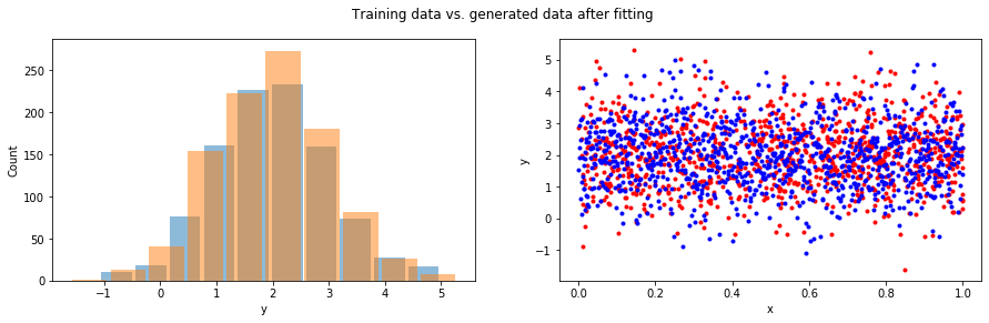
#     <tf.Variable 'Variable:0' shape=(1,) dtype=float32, numpy=array([1.0158775], dtype=float32)>)

fig = plt.figure(figsize=(15, 4))
fig.suptitle('Training data vs. generated data after fitting')

plt.subplot(1, 2, 1)
x = np.linspace(min(x_train), max(x_train), 1000)
y = tf.random.normal(shape=(len(x_train),), mean=gaussian_fit_layer.m, stddev=gaussian_fit_layer.s)
plt.hist(y, rwidth=0.9, alpha=0.5)
plt.hist(y_train, rwidth=0.9, alpha=0.5)
plt.xlabel('y')
plt.ylabel('Count');

plt.subplot(1, 2, 2)
plt.plot(x_train, y_train, 'r.')
plt.plot(x, y, 'b.');
plt.xlabel('x')
plt.ylabel('y');

In a future blog post, we will discuss how to structure our custom training loops so that we can use the tf.function decorator to speed things up!

How is mean squared error related to log-likelihood?

There is a fundamental mind-blowing connection between MSE and log-likelihood on a linear Gaussian model. Let us assume that our data are modelled by the linear model \(\mathbf{Y} = \mathbf{X} \mathbf{\Theta} + \epsilon\), where \(\epsilon_i \sim N(0,\sigma_e^2)\). Therefore:

\[\mathbf{Y} - \mathbf{X}\mathbf{\Theta} = \epsilon\]

And the log-likelihood is:

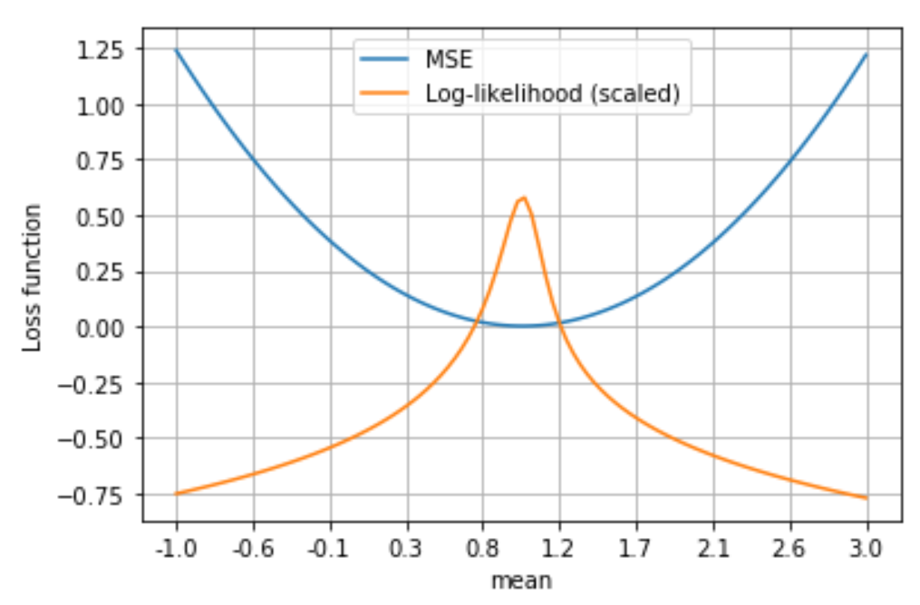
\[\begin{align*} \log \mathcal{L}(\mathbf{\Theta} \mid \mathbf{Y}, \mathbf{X}) &= \log\prod_{i=1}^N \text{PDF}(\epsilon_i)= \sum_{i=1}^N \log \text{PDF}(\epsilon_i)\\ &= \sum_{i=1}^N \log \left[ \frac{1}{\sqrt{2\pi \sigma_e^2}} \exp\left(-\frac{(\mathbf{Y}_i - \mathbf{X}_i \mathbf{\Theta})^2}{2\sigma_e^2}\right)\right]\\ &=-\frac{N}{2} \log \left( 2\pi \sigma_e^2 \right) - \sum_{i=1}^{N} \left( \frac{(\mathbf{Y}_i - \mathbf{X}_i \mathbf{\Theta})^2}{2\sigma_e^2}\right) \end{align*}\]

In order to maximize \(\log \mathcal{L}(\mathbf{\Theta} \mid \mathbf{Y}, \mathbf{X})\), we need to minimize \(\sum_{i=1}^{N} \left( -\frac{(\mathbf{Y}_i - \mathbf{X}_i \mathbf{\Theta})^2}{2\sigma_e^2}\right)\), but this is equivalent to minimizing \(N \cdot \text{MSE}\) or to minimizing MSE. In the following plot we see the values of log-likelihood and MSE for various values of the parameter \(\mu\) in a linear regression model. Notice how the value of \(\mu\) that minimizes MSE is the same that maximizes log-likelihood!