Why is normal distribution so ubiquitous?
machine learning Mathematica mathematics statisticsContents
- Introduction
- As simple as it can get
- Why is convolution the natural way to express the sum of two random variables?
- Information-theoretic arguments
- References
Many thanks to Alexander Nordin for spotting some errors in the combinations of four dice and being kind enough to let me know.
Introduction
Have you ever wondered why normal distributions are encountered so frequently in everyday life? Some examples include the height of people, newborns’ birth weight, the sum of two dice, and numerous others. Also, in statistical modeling, we often assume that some quantity is represented by a normal distribution. Particularly when we don’t know the actual distribution, but we do know the sample mean and standard deviation. It is as if Gaussian is the “default” or the most generic. Is there some fundamental reason Gaussians are all over the place? Yes, there is!

As simple as it can get
The case of rolling dice
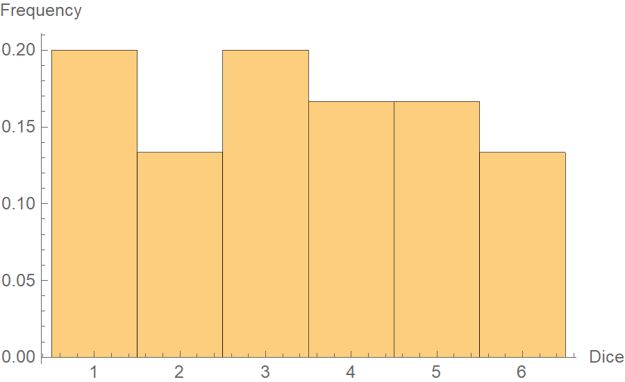
Let’s take a couple of examples, starting with the case of throwing a fair die. Every number on each marked side has an equal probability of showing up, i.e., p=1/6. Let us examine the following sequence of 30 trials:
3, 4, 6, 5, 1, 5, 6, 5, 1, 5, 3, 1, 2, 4, 1, 1, 2, 5, 3, 1, 3, 4, 3, 6, 2, 4, 6, 2, 4, 3If we get to plot the frequency histogram of these numbers, we notice something resembling a uniform distribution. Considering we only threw the die 30 times, the small deviations are ok.
Here comes the magic. Suppose that we throw two dice 15 times, and we get the follwing pairs:
{3, 4}, {6, 5}, {1, 5}, {6, 5}, {1, 5}, {3, 1}, {2, 4}, {1, 1},
 {2, 5}, {3, 1}, {3, 4}, {3, 6}, {2, 4}, {6, 2}, {4, 3}
So the first time, we get 3 and 4, the second time 6 and 5, and so on. Now let us take the sum of each pair:
7, 11, 6, 11, 6, 4, 6, 2, 7, 4, 7, 9, 6, 8, 7And let’s plot the frequency histogram of the sums.
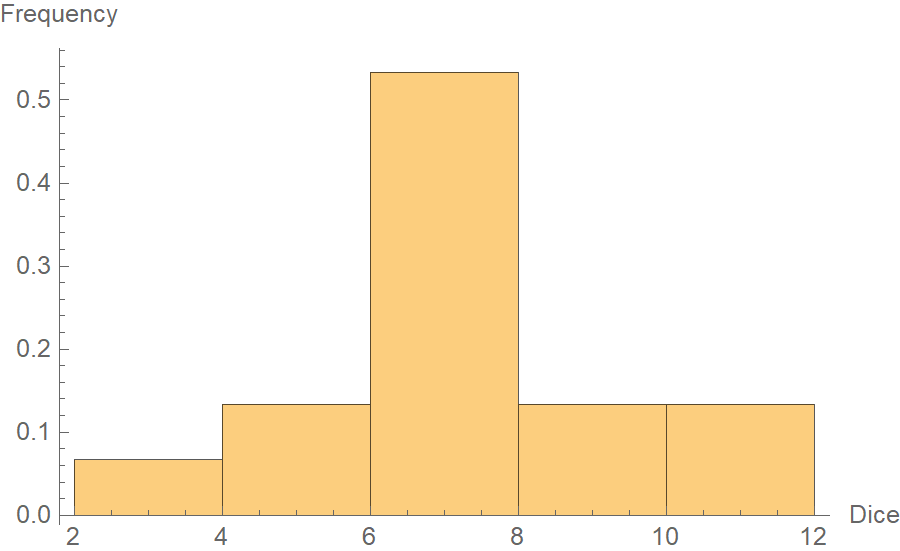
As you notice, the sums’ distribution switched from a uniform to something that starts looking like a Gaussian. Just think about it for a second. Why does the number 7 appear so often as the sum of two dice? Well, because many combinations could end up having a sum of 7. E.g., 1 + 6, 6 + 1, 2 + 5, 5 + 2, 3 + 4, 4 + 3. The same logic applies to 6 as well. However, to get some very large sum, say 12, there is only one combination, namely 6 + 6. The same applies to small sums, like 2, which is realized only by 1 + 1.
If we keep going by throwing more dice, say 4 at a time, the sums’ distribution will get even closer to a normal distribution. There will be even more combinations of dice outcomes summing up to a “central” value, rather than in some extreme value. In the following figure, we plot the number of distinct combinations that yield all possible sums in a “roll 4 dice” scenario. There is an exact correspondence between the number of generating combinations and the frequency a sum appears.
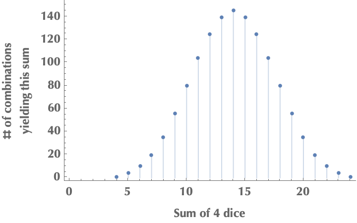
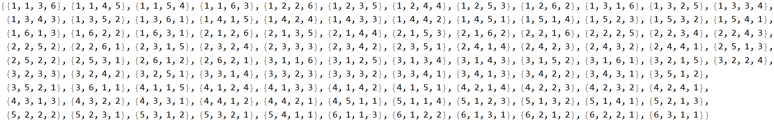
So here are the 104 combinations of dice values that sum to 11.
In the following histograms, we examine the sums’ distributions, starting with only one die and going up to 20 dice! By rolling merely three dice, the sum already looks pretty normally distributed.
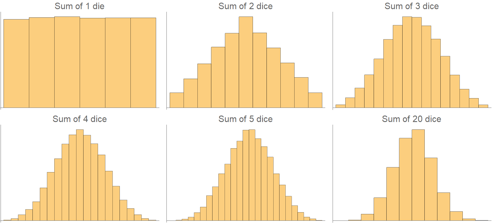
We may now answer why bell curves are so ubiquitous: because many variables in the real world are the sum of other independent variables. And, when independent variables are added together, their sum converges to a normal distribution. Neat?
The case of random walks
This example is reproduced (and modified) by the excellent book “Statistical Rethinking: A Bayesian Course with Examples in R and Stan; Second Edition”. Suppose we place 1000 folks on a field, one at a time. We then ask them to flip a coin and depending on the outcome, they take a step in the left or right direction. The distance of each step is a random number from 0 to 1 meter. Each person takes, say, a total of 16 such steps. The blue lines are the trajectories of the 1000 random walks. The red line is one such representative walk. At the right end of the plot, the grey line is the probability distribution of the position when the random walks have been completed.
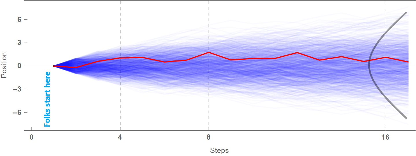
At the end of this game, we can’t really tell each person’s position, but we can say something about the distribution of their distances. Arguably, the distribution will look normal simply because there are vastly more sequences of left-right steps whose sum ends up being around zero than sequences of steps that end up being far away from zero. For example, to end up near position 6 or -6, one needs to take 16 consecutive left steps or 16 successive right steps. That’s just very unlikely to happen (remember that the direction people move is determined by a flip coin, so they should have 16 heads or 16 tails in a row). The following Mathematica code generates the plot below, but feel free to skip it.
randomWalks[reps_, steps_] :=
 Module[{},
  Table[
   Accumulate[
    Flatten@Append[{0},
      RandomVariate[UniformDistribution[{-1, 1}], steps]]],
   {k, reps}]
  ]

Show[
 ListPlot[walks, Joined -> True, PlotStyle -> Directive[Blue, Opacity[0.02]],
  AspectRatio -> 1/3, Frame -> {True, True, True, True}, FrameLabel -> {"Steps", "Position"},
  FrameTicksStyle -> Directive[Bold], FrameTicks -> {{{-6, -3, 0, 3, 6}, None},
   {{0, 4, 8, 16, 32}, None}},
  GridLines -> {{4, 8, 16, 32}, None}, GridLinesStyle -> Dashed, ImageSize -> Large],
 ListPlot[walks[[1]], Joined -> True, PlotStyle -> Red]]
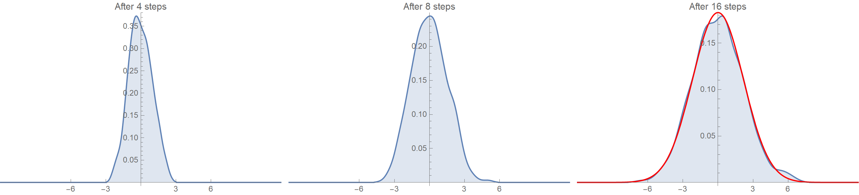
These are the distributions of the positions (distances) after 4, 8, and 16 steps. Notice how the distribution converges on a Gaussian (the red one) as the number of steps increases.
What we have discussed so far is the other side of the central limit theorem (CLT). CTL establishes that when independent random variables are added, their properly normalized sum converges toward a normal distribution even if the original variables themselves are not normally distributed.
The mind-blowing thing about this is that it doesn’t matter what the underlying distribution processes are. They might be uniform like in our examples, or (almost) anything else. In the end, the sums will converge on a Gaussian. The only thing that can vary is the speed of convergence, which is high when the underlying distribution is uniform and slower otherwise.
So why are normal distributions so ubiquitous?
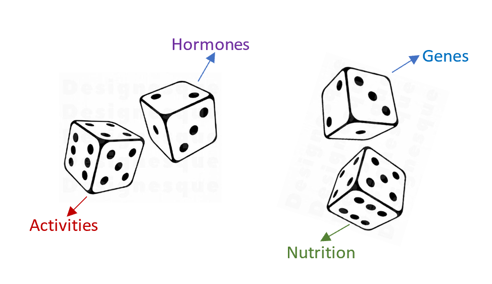
Because many things in our world emerge as the sum of smaller independent parts. For instance, consider a person’s height. This is determined by the sum of many independent variables:
- The genes (I haven’t researched it by I presume several genes contribute to height, not just one)
- Hormones (E.g., growth hormone)
- The environment
- The nutrition in terms of what one eats every day during the developmental phase
- Sports / activity levels
- Pollution
- Other factors
A person’s height is akin to the sum of rolling many dice. Each die parallels one of the above factors. I.e., the genes match the 1st die, the hormones the 2nd, etc. So, to end up being very tall, you need them all working in favor of you: the genes, the hormones, the environment, the activity, etc. It’s as if scoring 16 heads in a row in the random walk setting. That’s why there are few very tall people. The same logic applies to very short people. In this case, you need to have everything working against you: bad genes, poor nutrition, no activity, etc. However, most people have an average height because some factors contribute positively and others negatively.
What follows is the presentation of the same arguments with some math. Do not worry if you find them confusing. You won’t have missed any insights!
Why is convolution the natural way to express the sum of two random variables?
Summing random variables is at the heart of our discussion, so it deserves a few thoughts. Suppose that we have two random variables, \(X, Y\), and we take their sum, \(Z=X+Y\). Depending on what mathematical tools we use to describe the random variables, their sum is expressed differently. For a full list, feel free to check this link. We will discuss the case where \(X, Y, Z=X+Y\) all have a probability mass function (PMF).
By definition, a PMF is a function that gives the probability that a discrete random variable is exactly equal to some value. For a fair die, the PMF is simply \(p(x)=\text{Pr}(X=x_i)=1/6\), with \(x_i=\{1,2,\ldots,6\}\). Back to our sum \(Z=X+Y\). By definition, again, the PMF for \(Z=X+Y\) at some number \(z_i\) gives the proportion of the sum \(X+Y\) that is equal to \(z_i\) and is denoted as \(\text{Pr}(Z=z_i), z_i=X+Y\). By applying the Law of Total Probability, we can break up \(\text{Pr}(Z=X+Y)\), into the sum over all possible values of \(x\), such that \(X=x\), and \(Y=z-x\).
\[\text{Pr}(z=X+Y) = \sum_{x} \text{Pr}(X=x,Y=z−x)\]But, that’s the definition of the convolution operation in the discrete case. For continuous variables, it’s just:
\[(f \star g)(t) \stackrel{\text{def}}{=} \int_{-\infty}^\infty f(x) \, g(t - x) \, \mathrm{d}x\]Convolving a unit box
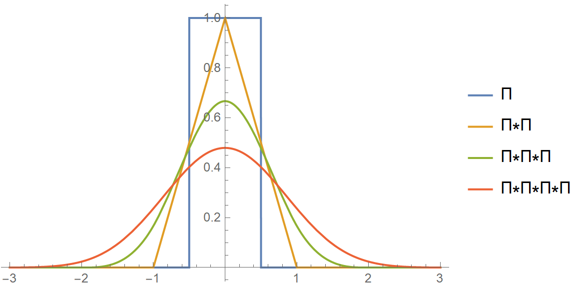
Let’s look at an example where we will convolve the unit box function with itself. The unit box function is equal to 1 for \(\mid x\mid \le 1/2\) and 0 otherwise.
f0[x_] := UnitBox[x];
fg[f_, g_] := Convolve[f, g, x, y] /. y -> x
(* Cache the results because symbolic convolution takes time *)
repconv[n_] := repconv[n] = Nest[fg[#, #] &, f0[x], n]
Grid[
 Partition[#, 2] &@
  (Plot[#, {x, -3, 3}, Exclusions -> None, Filling -> Axis] & /@
    Table[repconv[k], {k, 0, 3}])
 ]
The following animation might clear up the operation of convolution between two functions.
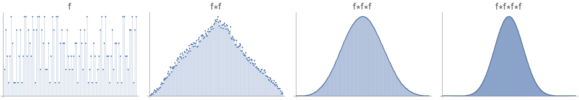
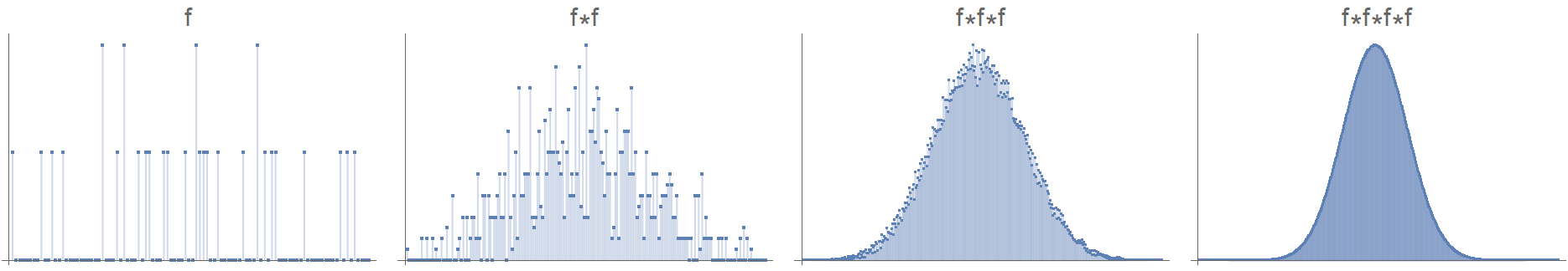
Convolving noisy data
Ok, so convolving a unit box function with itself, which pertains to rolling two dice and calculating their sums, led us to a Gaussian distribution. Does this have to do with the unit box? No! Αny distribution with a finite variance will morph into a Gaussian, given some time and repeated convolutions. In the following examples, we start with some quite noisy initial distributions and convolve them repeatedly with themselves. As you see, the result is again a normal distribution!
Information-theoretic arguments
In 1948 Claude Shannon laid out the foundations of information theory. The need this new theory was called upon to meet was the effective and reliable transmission of messages. Although the motive was applied, information theory is deeply mathematical in its nature. A central concept in it is entropy, which is used somewhat differently than in thermodynamics. Consider a random variable \(X\), which assumes the discrete values \(X = \{x_i \mid i=1, 2, \ldots, K\}\). Of course, \(0 \le p_i \le 1\) and \(\sum_{i=1}^{K} p_i = 1\) must also be met.
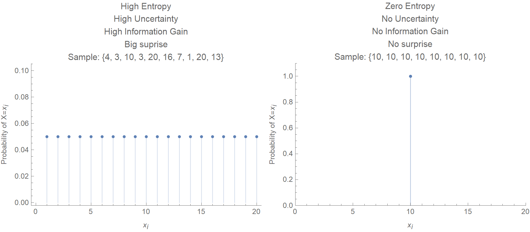
Consider now the extreme case where the value \(X=x_i\) has a probability of occurring \(p_i=1\), and \(p_{j\ne i}=0\). In this scenario, there’s no “surprise” in observing the value of \(X\), and there’s no message being transmitted. It is as if I told you that it’s chilly today in Alaska or that sun raised at east. In this context, we define the information content that we gain by observing \(X\) as the following function:
\[I(x_i) = \log\left(\frac{1}{p_i}\right) = -\log p_i\]We then define as entropy the expected value of \(I(x_i)\) over all \(K\) discrete values \(X\) takes:
\[H(X) = \mathop{\mathbb{E}} \left(I(x_i)\right) = \sum_{i=1}^{K} p_i I(x_i) = \sum_{i=1}^{K} p_i \log\frac{1}{p_i} = -\sum_{i=1}^{K} p_i \log p_i\]Here we compare two discrete probability distributions, one with high entropy and the other with zero entropy.
Similarly, we define differential entropy for continuous variables:
\[h(X) = -\int_{-\infty}^{\infty} p_X(x) \log p_X(x) \mathrm{d}x\](However, some of the discrete’s entropy properties do not apply to differential entropy, e.g., differential entropy can be negative.)
Alright, but what normal distribution has anything to do with these? It turns out that normal distribution is the distribution that maximizes information entropy under the constraint of fixed mean \(m\) and standard deviation \(s^2\) of a random variable \(X\). So, if we know the mean and standard deviation of some data, out of all possible probability distributions, Gaussian is the one that maximizes information entropy, or, equivalently, it is the one that satisfies the least of our assumptions/biases. This principle may be viewed as expressing epistemic modesty or maximal ignorance because it makes the least strong claim on a distribution.
A discrete distribution with support {0,1}
Let us take a look at a very simple setup. E.g., consider a coin that comes tails with a probability \(p\), and heads with a probability \(1-p\). The entropy of the flip is then given by:
\[H(X) = - \sum_{i=1}^2 p_i \log p_i = -p \log p - (1-p) \log (1-p)\]Here is the plot of entropy \(H(p)\) vs. probability \(p\). Notice how entropy is maximized when we assume that the coin is fair, i.e., \(p=0.5\).
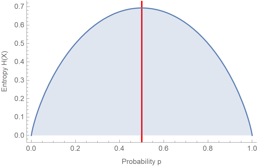
Let us solve it analytically, by taking the derivative of entropy and setting it equal to zero:
\[\begin{aligned} H(p) &=-p \log p-(1-p) \log (1-p) \\ \frac{\partial H}{\partial p} &=-\log p-1+\log (1-p)+1 =\log \frac{1-p}{p} \\ \frac{\partial H}{\partial p} &=0 \Leftrightarrow \log \frac{1-p}{p}=0 \Leftrightarrow \frac{1-p}{p}=1 \Leftrightarrow p=\frac{1}{2} \end{aligned}\]So, in the absence of any data suggesting otherwise, such as that the coin is biased, the most honest position to take is to assume that all outcomes are equally probable. Consider the principle of maximum entropy as a form of “presumption of innocence”. ;)
A discrete distribution with support {a, …, b}
In this case the random variable \(X\) takes the values \(\{a,a+1,\ldots,b-1,b\}\), with probabilities \(\{p_a, p_{a+1} \ldots, p_{b-1}, p_b\}\). The entropy is equal to:
\[\begin{aligned} H(X)=-\sum_{i=a}^{b} p_{i} \log p_i \end{aligned}\]The only constraint we impose is that \(\sum_{i=a}^{b} p_{i}=1\). We write the Lagrangian and take the partial derivatives:
\[\begin{aligned} \mathcal{L}\left(p_{i}, \lambda\right)&=-\sum_{i=a}^{b} p_{i} \log p_{i}-\lambda\left(\sum_{i=a}^{b} p_{i}-1\right) \\ \frac{\partial \mathcal{L}}{\partial p_{i}}&=-\sum_{i=a}^{b}\left(\log p_{i}+1\right)-\lambda\left(\sum_{i=a}^{b} 1\right)= \\ &=-\left(\log p_{i}+1\right)(b-a+1)-\lambda(b-a+1) \\ \frac{\partial \mathcal{L}}{\partial \lambda}&=-\left(\sum_{i=a}^{b} p_{i}-1\right) \end{aligned}\]We solve for the stationary points of the Lagrangian \(\mathcal{L}\):
\[\begin{aligned} \frac{\partial \mathcal{L}}{\partial p_{i}}&=-\log p_i-1-\lambda=0 \Leftrightarrow p_{i}=e^{-1-\lambda}\\ \frac{\partial \mathcal{L}}{\partial \lambda}&=0 \Leftrightarrow \sum_{i=a}^{b} p_{i}=1 \Rightarrow \sum_{i=a}^{b}\left(e^{-1-\lambda}\right)=1 \\ & \Leftrightarrow e^{-1-\lambda}(b-a+1)=1\\ & \Leftrightarrow \lambda=\log(b-a+1)-1 \end{aligned}\]Therefore the probability is equal to:
\[p_i = \frac{1}{b-a+1}\]So basically, this case is a generalization of the previous. For \(a=0, b=1\), we get the probability of the fair coin.
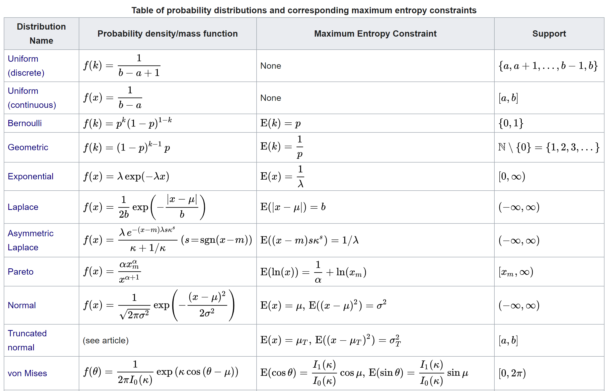
Edwin Thompson Jaynes put it very beautifully that the max entropy distribution is “uniquely determined as the one which is maximally noncommittal with regard to missing information, in that it agrees with what is known, but expresses maximum uncertainty with respect to all other matters”. Therefore, this is the most principled choice. Here is a list of probability distributions and their corresponding maximum entropy constraints, taken from Wikipedia.
References
- Statistical Rethinking: A Bayesian Course with Examples in R and Stan; Second Edition, by Richard McElreath.
- Neural Networks and Learning Machines 3rd Edition, by Simon Haykin.