An introduction to Gaussian Processes
machine learning Mathematica mathematics regression statisticsContents
- Introduction
- The ingredients
- A simple 1D GP prediction example
- Limitations of Gaussian Processes
- References
Introduction
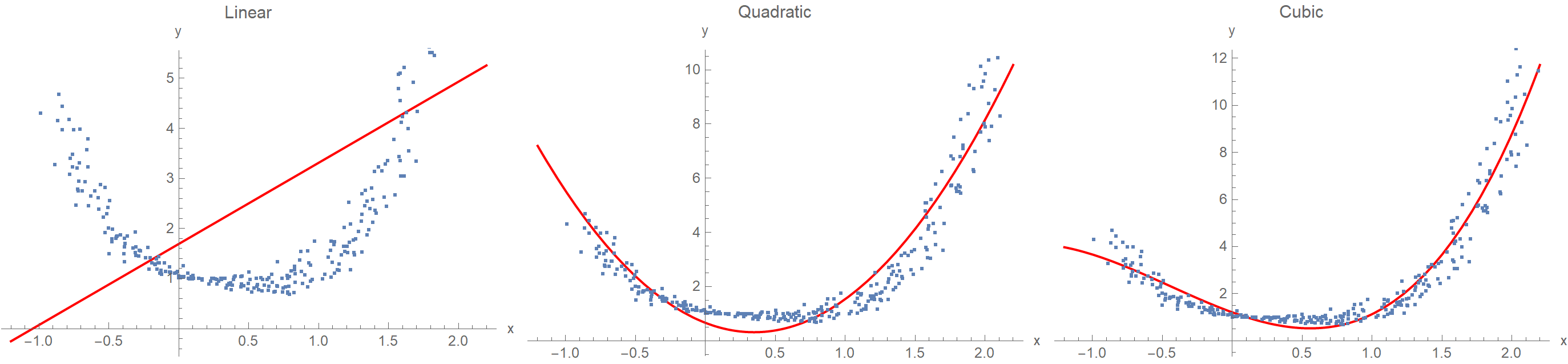
One of the recurring topics in statistics is establishing a relationship between a response variable \(y\) and some predictor variable(s) \(x\), given a set of data points. This procedure is known as regression analysis and is typically done by assuming a polynomial function whose coefficients are determined via ordinary least squares. But what if we don’t want to commit ourselves upfront on the number of parameters or even the functional form to use? Suppose we’d like to consider every possible function as a candidate model for our data. That’s bold, but could we pull it through? The answer is yes, with the help of Gaussian Processes (GP).
The ingredients
Gaussian process priors
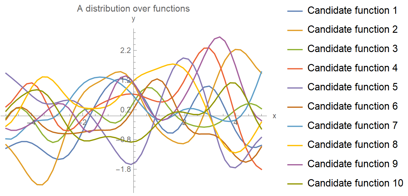
Let’s start with a distribution of all possible functions that, conceivably, could have produced our data (without actually looking at the data!). This is portrayed in the following plot, where we have drawn 10 such candidate random functions. In principle, the number is infinite, but for brevity, we only drew 10 here. These functions are known as GP priors in the Bayesian vernacular. They capture our ignorance regarding the true generating function \(y = f(x)\) we are after.
From GP priors to GP posteriors
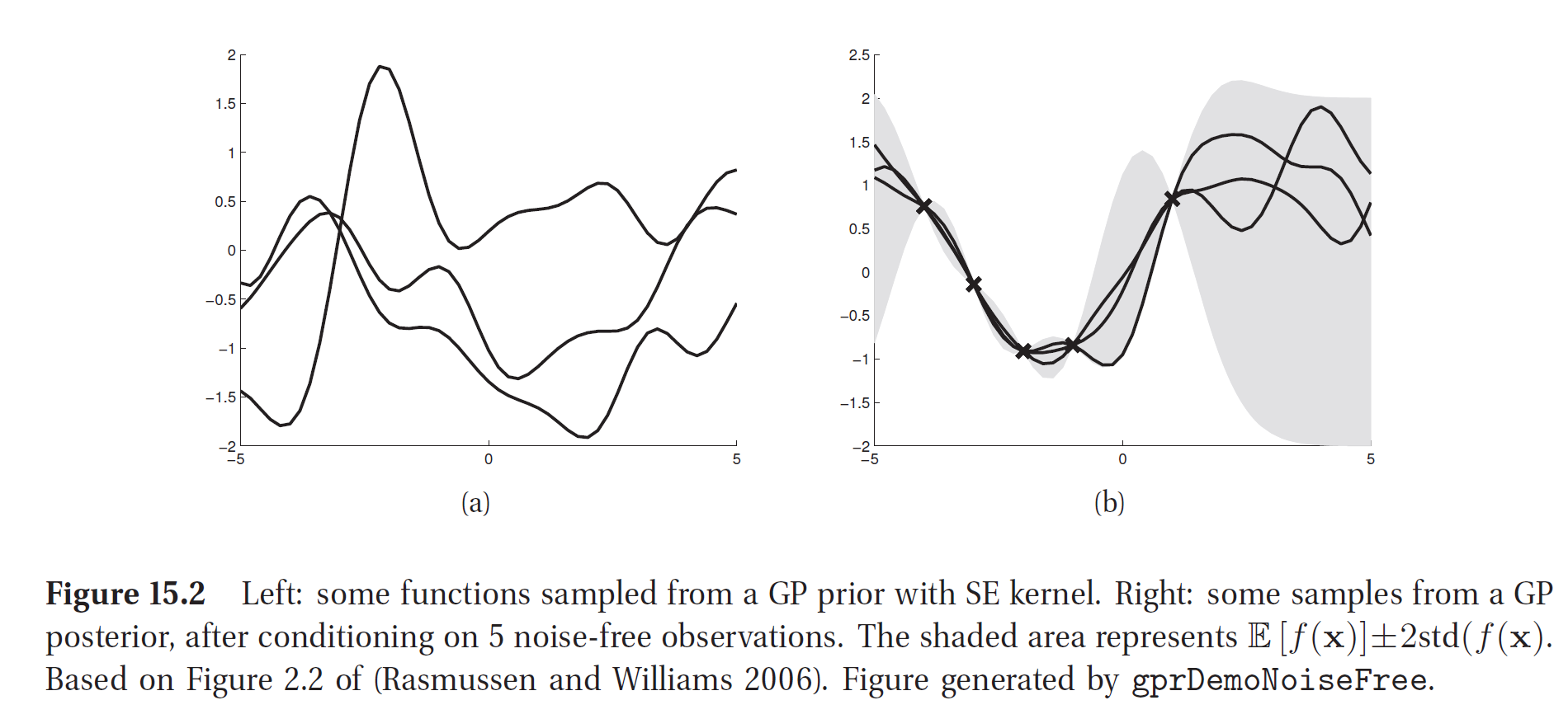
Then, as we look at the data, we narrow down the functions that could have generated them. In the following example, after considering 5 observations, we build-up some pretty strong confidence regarding how the data-generating function should look like. It’s as if we put a vertical loop around the prior functions at the training data points, and then we pull the rope. The shaded area represents our model’s uncertainty, being high where we lack data and low where we have many data points. The image was taken from the book Machine Learning A Probabilistic Perspective by Kevin P. Murphy, which is very nice, by the way.
Constraining the priors
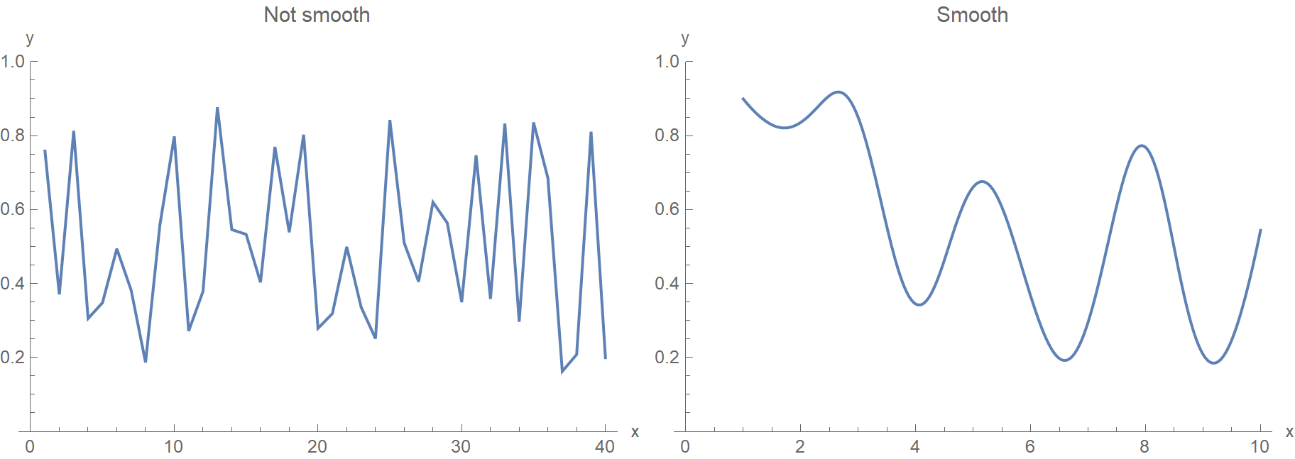
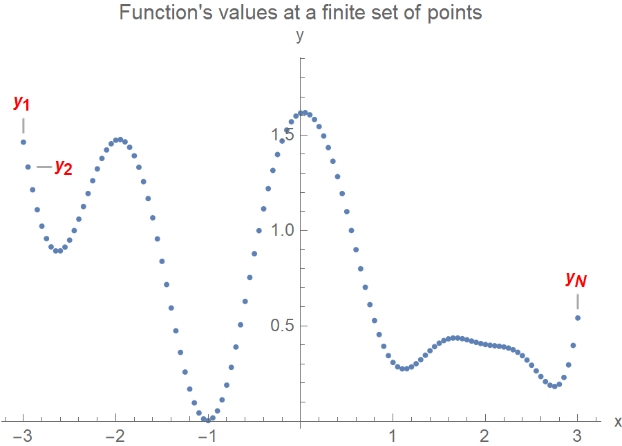
The truth is that we don’t really want to consider every mathematically valid function. Instead, we need to impose some constraints on the prior distribution over all possible functions. For starters, we want our functions to be smooth because this matches our empirical knowledge about how the world generally works. Points that are close to each other in the input space (whether in the time domain, i.e. \(t_1, t_2, \ldots\) or in the spatial domain, i.e. \(x_1, x_2, \ldots\)) are associated with \(y_1, y_2, \ldots\) values that are also close to each other. Therefore, we don’t really want our algorithm to favor solutions that look like the left edgy function.
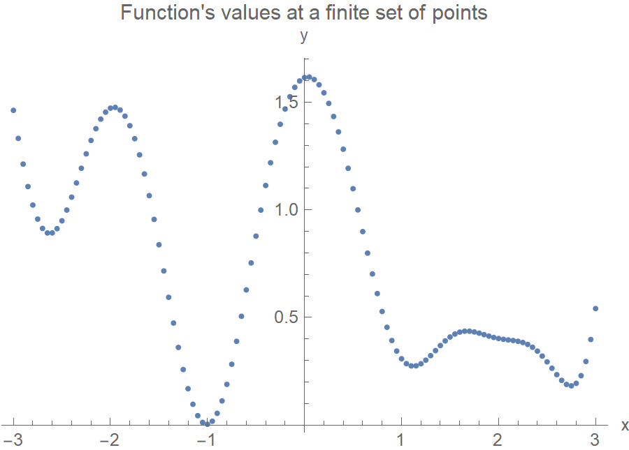
Which brings us to the following question: how do we introduce smoothness? Although we talk about the distribution over functions, in reality, we define the distribution over the function’s values at a finite yet arbitrary set of points, say \(x_1, x_2, \ldots, x_N\). I.e., we model functions as really long column vectors. You also need to realize that every point \(y_1, y_2, \ldots, y_N\) is treated as a random variable, and the joint probability distribution of \(p(y_1, y_2, \ldots, y_N)\) is a multivariate normal distribution (MVN). Let that sink in for a moment because this is the heart of GP. To generate the following function, we set up a 120-variate normal distribution and take a single 120-variate sample from it. This 120 long \(y\) vector corresponds to our function.
Ok, but if we sample from a 120-variate Gaussian, how can we guarantee the function’s smoothness? After all, the \(y_i\)’s are random! First, to set up a 120-variate Gaussian, we need a 120x120 covariance matrix. Each element of the matrix determines how much the \((y_i, y_j)\) variables are related. The trick now is to use a covariance matrix such that the values that are close in the input space, the \(x\)’s, will produce values that are close in the output space, the \(y\)’s. In the following plot, \(x_1\) and \(x_2\) are close together, so we’d expect \(y_1\) and \(y_2\) to also be close (this makes the function smooth and not too wiggly). On the contrary, \(x_1\) and \(x_N\) are very apart, so the covariance matrix element \(\Sigma_{1N}\) should be some tiny number. And \(y_1, y_N\) would be allowed to be as far away as they’d feel like.
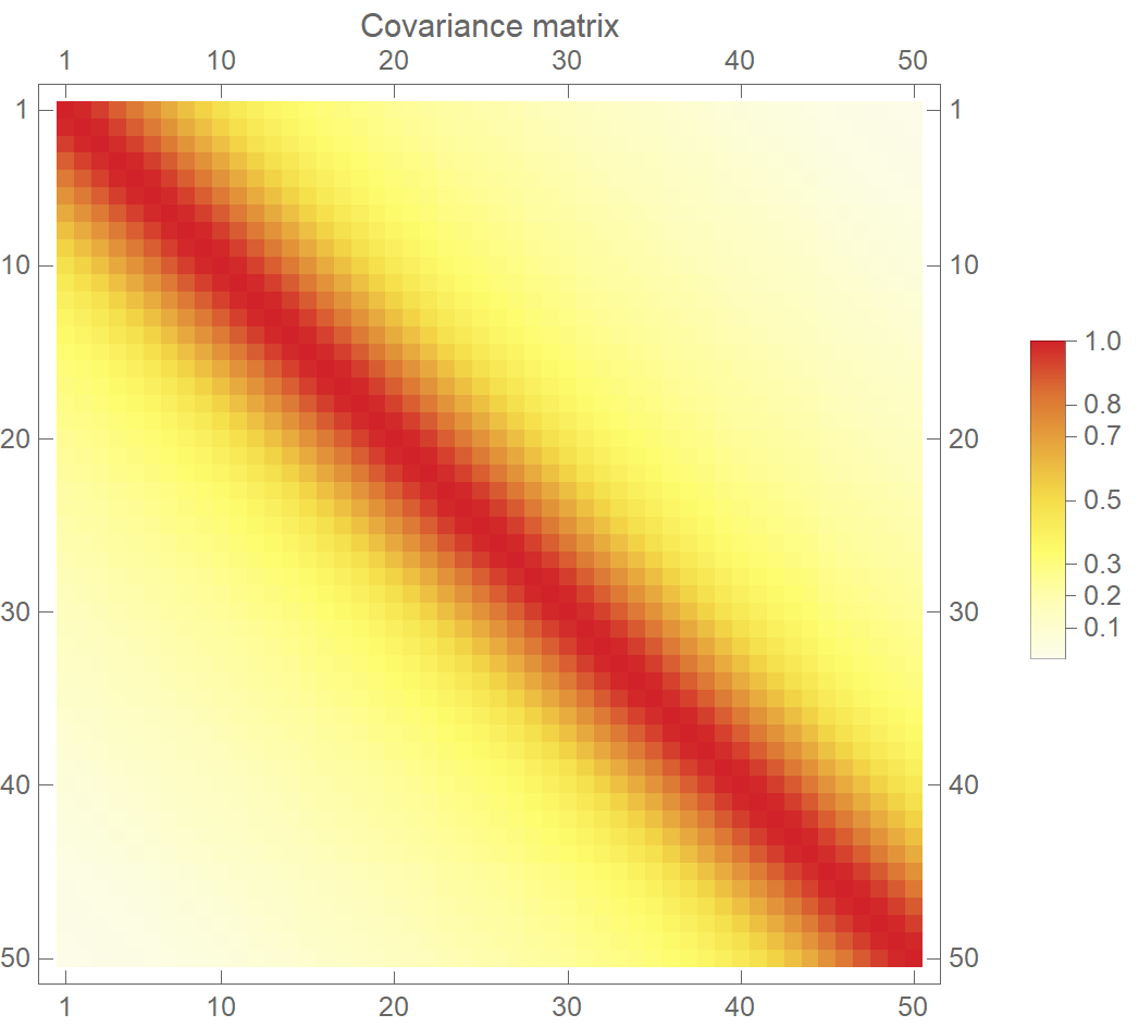
In the following plot, we visualize such a legitimate covariance matrix. The variables near the diagonal, i.e., variables close in the input space, are assigned a high value (\(\Sigma_{ij}=1\)). Therefore, when we sample from the multivariate normal distribution, these points will come out as neighbors. On the contrary, the rest of the pairs are given a low value (\(\Sigma_{ij}=0\)). Hence, when we sample from the MVN, the \(y\)’s will be uncorrelated. Alright, but how do we actually calculate the values of the covariance matrix? We use a specialized function called kernel (also known as covariance function).
A kernel function is just a fancy name for a function that accepts as input two points in the input space, i.e., \(x_i\) and \(x_j\), and outputs how “similar” they are based on some notion of “distance”. For example, the following kernel is the exponentiated quadratic that uses the exponentiated squared Euclidean distance between two points. If \(x=x'\), then \(k(x, x') = \exp(0)=1\), whereas if \(\|x-x'\| \to \infty\), then \(k(x, x') \to 0\).
\[k(x,x') = \sigma^2 \exp\left(-\frac{1}{2\ell^2}\|x-x'\|^2\right)\]The \(\ell\) parameter determines the length of the “wiggles”. Generally speaking, we won’t be able to extrapolate more than \(\ell\) units away from our data. Similarly, the variance \(\sigma^2\) determines the average distance of our function from its mean value. In short, \(\ell, \sigma\) circumscribe the horizontal and vertical “range” of the function. As you may have guessed, they are indeed hyperparameters (i.e., their values need to be set by us; they can’t be inferred automatically by the algorithm). The following image shows various different kernels that can be used in GP and the derived GP priors. By the way, the same kernels are also used in Support Vector Machines (SVM).
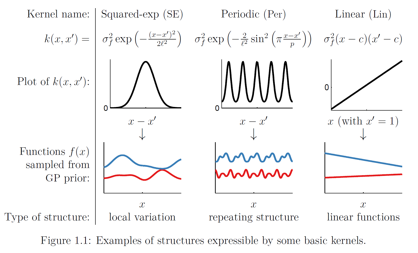
Image taken from here.
Given a kernel \(k(x,x')\) we construct the covariance matrix with:
\[\Sigma(x,x')= \begin{bmatrix} k(x_1,x_1) & k(x_1,x_2) & k(x_1,x_3) & \dots & k(x_1,x_N) \\ k(x_2,x_1) & k(x_2,x_2) & k(x_2,x_3) & \dots & k(x_2,x_N) \\ \vdots & \vdots & \vdots & \vdots & \vdots\\ k(x_N,x_1) & k(x_N,x_2) & k(x_N,x_3) & \dots & k(x_N,x_N) \\ \end{bmatrix}\]The covariance matrix \(\Sigma(x,x')\) must be positive definite, meaning that the following condition must be met:
\[x^⊤ \Sigma x > 0, \forall x \ne 0\]This is the multivariate analog of the univariate requirement for the variance \(\sigma^2\) to be positive. Although we haven’t made any reference to it, we also need a mean function \(m(x)\) to fully characterize the MVN that we will be sampling our \(y\)’s from. Having all the ingredients in place, we write:
\[Y(x) \sim \mathcal{GP}\left(m(x),k(x,x')\right)\]Making predictions from Gaussian Processes posteriors
We have gone through all the fuzz to make some predictions. Right? So, suppose that we have \(n_1\) new testing samples, and we are going to base these predictions on \(n_2\) previously observed data points. Keep in mind that both the training and testing \(y\)’s (that we want to calculate) are jointly Gaussian, since they both come from the same MVN. Having said that and given samples’s finite size we can write:
\[Y = \left( \begin{array}{c} Y_1 \\ Y_2 \end{array} \right) \quad \mbox{ with sizes } \quad \left( \begin{array}{c} n_1 \times 1 \\ n_2 \times 1 \end{array} \right)\] \[\mu = \left( \begin{array}{c} \mu_1 \\ \mu_2 \end{array} \right) \quad \mbox{ with sizes } \quad \left( \begin{array}{c} n_1 \times 1 \\ n_2 \times 1 \end{array} \right)\] \[\Sigma = \left(\begin{array}{cc} \Sigma_{11} & \Sigma_{12} \\ \Sigma_{21} & \Sigma_{22} \end{array} \right) \ \mbox{ with sizes } \ \left(\begin{array}{cc} n_1 \times n_1 & n_1 \times n_2 \\ n_2\times n_1 & n_2\times n_2 \end{array} \right)\]Just to make sure that we are on the same page here: \(Y_1\) contains the \(y\) values we want to calculate, \(Y_2\) contains the \(y\) values from the training set, \(\Sigma_{11}\) is the covariance matrix for the testing set, \(\Sigma_{22}\) for the training set and \(\Sigma_{12} = \Sigma_{21}\) for the mixed testing-training set. The distribution of \(Y_1\) conditional on \(Y_2=y_2\) is \(Y_1 \mid y_2 \sim \mathcal{N} (\bar{\mu}, \bar{\Sigma})\), where:
\[\begin{align} \bar{\mu} &= \mu_1 + \Sigma_{12} \Sigma_{22}^{-1}(y_2 - \mu_2) \\ \mbox{and } \quad \bar{\Sigma} &= \Sigma_{11} - \Sigma_{12} \Sigma_{22}^{-1} \Sigma_{21} \end{align}\]If you feel like reading more regarding conditional distributions, you can start here.
A simple 1D GP prediction example
Let us consider a somewhat contrived one-dimensional problem. The response variable \(y\) is a sinusoid measured at eight equally spaced \(x\) locations in the span of a single period \([0, 2\pi]\). This example is taken from here, and we reimplement it with Mathematica (the original implementation is in R).
ClearAll["Global`*"];

(* Define a squared exponential kernel *)
 kernel[a_, b_] := Exp[-Norm[(a - b), 2]^2]

(* These are our training data *)
nTrainingPoints = 8;
X = Array[# &, nTrainingPoints, {0, 2 Pi}];
Y = Sin[X];

eps = 10^-6;
Sigma = Outer[kernel, X, X] + eps*IdentityMatrix[nTrainingPoints];

nTestPoints = 100;
XX = Array[# &, nTestPoints, {-0.5, 2 Pi + 0.5}];

SigmaXX = Outer[kernel, XX, XX] + eps*IdentityMatrix[nTestPoints];
SigmaX = Outer[kernel, XX, X];
SigmaInverse = Inverse[Sigma];
Sigmap = SigmaXX - SigmaX . SigmaInverse . Transpose[SigmaX];

(* Although it is positive definite, it isn't symmetric due to small round off errors *)
{PositiveDefiniteMatrixQ[Sigmap], SymmetricMatrixQ[Sigmap]}
(* {True, False} *)

(* Make it symmetric *)
Sigmap = (Sigmap + Transpose@Sigmap)/2;
{PositiveDefiniteMatrixQ[Sigmap], SymmetricMatrixQ[Sigmap]}
(* {True, True} *)

mup = SigmaX . SigmaInverse . Y;

nsamples = 100;
YY = RandomVariate[MultinormalDistribution[mup, Sigmap], nsamples];
Dimensions@YY
(* {100, 100} *)

(* Calculate 5% and 95% quantiles for uncertainty modeling *)
quantiles = Transpose@Quantile[
    RandomVariate[
        MultinormalDistribution[mup, Sigmap], nsamples],
    {0.05, 0.95}];
Dimensions@quantiles
(* {2, 100} *)

Show[
    Table[
        ListPlot[Transpose@{XX, YY[[i]]}, AxesLabel -> {"x", "y"},
        Joined -> True, PlotStyle -> Opacity[0.1],
        PlotRange -> {Automatic, {-2, 2}}], {i, 1, nsamples}],
    ListPlot[Transpose@{XX, Mean[YY]}, AxesLabel -> {"x", "y"},
        Joined -> True, PlotRange -> {Automatic, {-2, 2}},
        PlotStyle -> Magenta],
    Plot[Sin[x], {x, -0.5, 2 \[Pi] + 0.5}, PlotStyle -> Black],
    ListPlot[Transpose@{XX, quantiles[[1]]}, PlotStyle -> {Red, Dashed}, Joined -> True],
    ListPlot[Transpose@{XX, quantiles[[2]]}, PlotStyle -> {Red, Dashed}, Joined -> True],
    ListPlot[Transpose@{X, Y}, PlotStyle -> {Blue, AbsolutePointSize[7]}]]
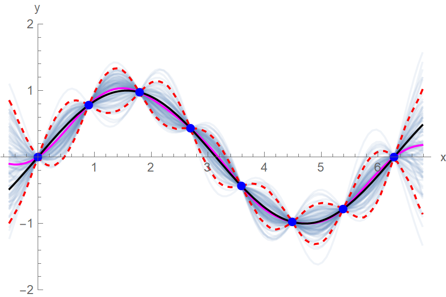
The blue points are the training data points, the black line is the ground truth function, the magenta line is our approximation after averaging 100 function samples, the red dotted lines are the 5% and 95% quantiles and the faded out blue lines are the 100 function realizations that we sampled from the MVN.
Limitations of Gaussian Processes
- Slow inference. Computing the covariance matrix’s inverse has a \(\mathcal{O}(N^3)\) time complexity, rendering exact inference too slow for more than a few thousand data points.
- Choosing a covariance kernel. There’s some arbitrariness when choosing a kernel. However, the kernel’s hyperparameters can be inferred by maximizing the marginal likelihood, and the whole process can be automated.
- Gaussian processes are in some sense idealizations. For the understanding of extreme phenomena exhibited by real physical systems, non-Gaussian processes might turn out more suitable. In this context, GPs serve as starting points to be perturbed.
References
- Surrogates: Gaussian process modeling, design and optimization for the applied sciences by Robert B. Gramacy, 2021-02-06. https://bookdown.org/rbg/surrogates/
- Machine Learning A Probabilistic Perspective by Kevin P. Murphy.