Python decorators and the tf.function
machine learning Python TensorflowContents
Python decorators
A decorator is a function that accepts another function as an argument and adds new functionality to it. Decorators are used for all sorts of things, like logging, timing the execution of functions, and caching values. Let’s see a couple of examples!
The most useless decorator
Arguably, the most useless decorator is the following one that does absolutely nothing! :)
def noop_decorator(func):
    return func

# The typical place to put a decorator is
# just before the definition of a function
@noop_decorator
def hello_world():
    return "Hello, world!"

hello_world()
#    Hello, world!
So, basically, the noop_decorator returns whatever function we hand it over, without modifying it at all.
Timing the execution of a function
In the following example, we construct a decorator called mytimer that prints the time in seconds a function takes to execute. The decorator accepts as input the function func and returns another function called wrapper. So, every time we call the calc_stuff() function, in reality the wrapper() function is executed. The latter saves the current value of a performance counter. It then uses the *args and **kwargs to collect the positional and keyword arguments. Subsequently, it runs the function func by forwarding the args and kwargs with the unpacking operators (asterisk and double asterisk). Next, it takes the difference between the new minus the old value of the performance counter and prints the result. This is the time elapsed during the execution of func. Finally, it returns the result of func, as we would expect if we had called the undecorated function.
import time

def mytimer(func):
    def wrapper(*args, **kwargs):
        start = time.perf_counter()
        func_value = func(*args, **kwargs)
        run_time = time.perf_counter() - start
        print(f'Function {func.__name__!r} in {run_time:.4f} secs')
        return func_value
    return wrapper

@mytimer
def calc_stuff(n):
    for _ in range(n):
        sum([i/3.14159 for i in range(2000)])
import timeit
timeit.timeit(lambda: calc_stuff(2000), number=10)
# Function 'calc_stuff' in 0.5119 secs
# Function 'calc_stuff' in 0.4639 secs
# Function 'calc_stuff' in 0.4689 secs
# Function 'calc_stuff' in 0.5194 secs
# Function 'calc_stuff' in 0.5252 secs
# Function 'calc_stuff' in 0.4812 secs
# Function 'calc_stuff' in 0.4630 secs
# Function 'calc_stuff' in 0.5072 secs
# Function 'calc_stuff' in 0.4528 secs
# Function 'calc_stuff' in 0.4544 secs
# 4.853907419000052Summing up the individual execution times, we get a total of 4.85 seconds, which is pretty close to the cumulative time timeit() reports. Next, we redefine the function with no decorator, and we notice how each function call’s execution time is gone now.
def calc_stuff(n):
    for _ in range(n):
        sum([i/3.14159 for i in range(2000)])

timeit.timeit(lambda: calc_stuff(2000), number=10)

#    4.638937220999992
Retrieving the lost metadata
When we decorate a function, we basically replace it with another function. This has the undesired side effect that some of the original function’s metadata are lost since they are replaced by the wrapper’s. See, for instance, the following code:
def noop_decorator(func):
    def wrapper(*args, **kwargs):
        """Just a wrapper function"""
        func_value = func(*args, **kwargs)
        return func_value
    return wrapper

@noop_decorator
def hello_world():
    """Returns the string Hello, world!"""
    return "Hello, world!"

@noop_decorator
def bye_world():
    """Returns the string Bye, world!"""
    return "Bye, world!"

[hello_world.__name__, bye_world.__name__]

#    ['wrapper', 'wrapper']
The same applies for the docstrings:
[hello_world.__doc__, bye_world.__doc__]
#    ['Just a wrapper function', 'Just a wrapper function']
To preserve the original function’s metadata, we use the functools.wraps(), which copies the metadata to the wrapper function that would be otherwise lost!
import functools

def noop_decorator(func):
    @functools.wraps(func)
    def wrapper(*args, **kwargs):
        """Just a wrapper function"""
        func_value = func(*args, **kwargs)
        return func_value
    return wrapper

@noop_decorator
def hello_world():
    """Returns the string Hello, world!"""
    return "Hello, world!"

@noop_decorator
def bye_world():
    """Returns the string Bye, world!"""
    return "Bye, world!"

[hello_world.__name__, bye_world.__name__]

#    ['hello_world', 'bye_world']
Neat! The function names were copied over. The same applies to the docstrings:
[hello_world.__doc__, bye_world.__doc__]

#    ['Returns the string Hello, world!', 'Returns the string Bye, world!']
Notice that although we had a docstring for the wrapper function, it was replaced by the original functions’ docstrings. Last, to blow your mind, functools.wraps is in itself a decorator! :P
Eager vs. lazy Tensorflow’s execution modes
Basic computation model
In Tensorflow, computations are modeled as a directed graph. Each node in the graph is a mathematical operation (say an addition of two scalars or a multiplication of two matrices). Every node has some inputs and outputs, possibly even zero. Along the edges of the graph, tensors flow! :) Tensors are multidimensional arrays with a specific type (e.g., float or double, etc.) and should not be confused with tensors in mathematical physics. For example, the mathematical operation \(\mathbf{\text{Relu}}\left(\mathbf{W} \mathbf{x} + \mathbf{b}\right)\) is represented as:
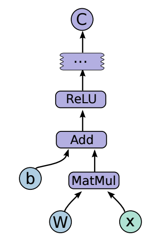
Image taken from here.
Tensorflow 1.0 and lazy execution
In Tensorflow 1.0, one had to construct the computation graph, then set up a session.run() with feed_dict to populate the graph with actual data. The advantage of working with a computation graph is that it allowed Tensorflow to perform many optimizations (e.g., graph simplifications, inlining function bodies to accommodate interprocedural optimizations, and so on). As of the time of writing, Grappler is the default graph optimization engine in the Tensorflow runtime. Grappler rewrites the graphs in order to improve performance, and also provides a plugin interface to register custom-made optimizers. A very basic example of such a simplification is the following algebraic one, that takes into account the properties of commutativity, assosiativity and distributivity:
\[2\mathbf{A} + 3 \mathbf{B} + 3 \mathbf{C} + \mathbf{\text{Identity}}(\mathbf{A}) \Rightarrow 3\mathbf{A} + 3 \mathbf{B} + 3 \mathbf{C} \Rightarrow 3 \text{tf.raw_ops.AddN}(\mathbf{A},\mathbf{B},\mathbf{C})\]Despite the speed benefits, though, Tensorflow’s 1.0 user experience left much to be desired, so eager execution mode was eventually introduced.
Tensorflow 2.0 and eager execution
In eager execution, we write some code, and we can run it immediately, line by line, examine the output, modify it, re-run it, etc. Everything is evaluated on the spot without constructing a computation graph that will be run later in a session. This is easier to debug and feels like writing regular Python code. Compare the following code:
# TensorFlow 2.x with eager execution (default)
import tensorflow as tf
a = tf.constant([[1, 2], [3, 4]])
b = tf.constant([[1, 2], [3, 4]])
print(a + b)
# tf.Tensor(
# [[2 4]
# [6 8]], shape=(2, 2), dtype=int32)
# Tensorflow 2.x with lazy execution
tf.compat.v1.disable_eager_execution()
a = tf.constant([[1, 2], [3, 4]])
b = tf.constant([[1, 2], [3, 4]])
print(a + b)
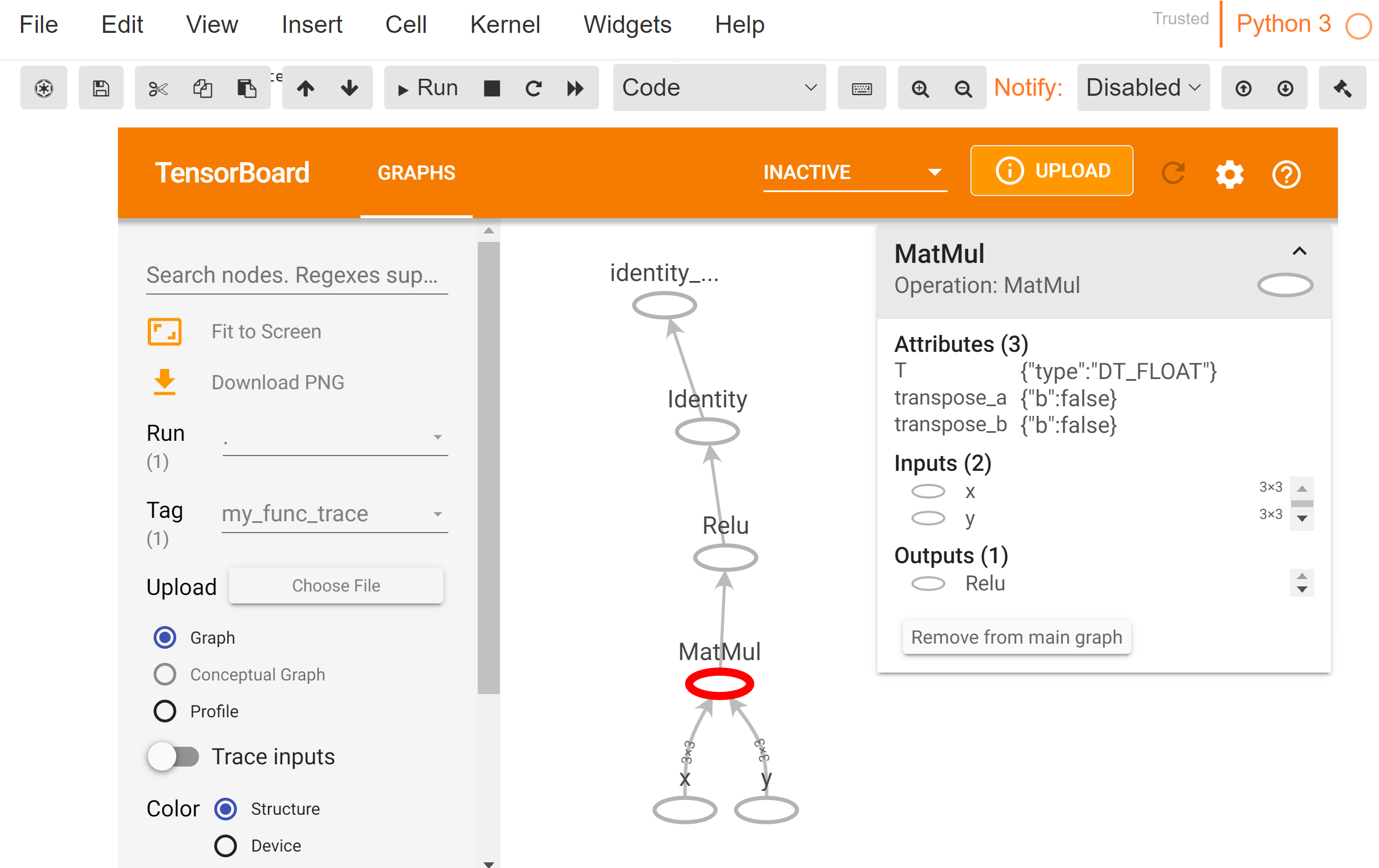
# Tensor("add:0", shape=(2, 2), dtype=int32)However, by running Tensorflow one step at a time, we give up the previous speed optimizations that were possible during the lazy execution mode. In Tensorflow 2.0, the default execution mode has been set to eager, presumably after people started to favor Pytorch over TF since Pytorch was eager from the beginning. So, where does the tf.function fit in this narrative? By using the tf.function decorator, we can convert a function into a Tensorflow Graph (tf.Graph) and lazy execute it, so we bring back some of the speed acceleration we gave up before. The following code uses the tf.function decorator to convert my_func() into a callable Tensorflow graph that we visualize with Tensorboard.
import tensorflow as tf

# The function to be traced
@tf.function
def my_func(x, y):
  return tf.nn.relu(tf.matmul(x, y))

# Set up logging
logdir = 'logs/'
writer = tf.summary.create_file_writer(logdir)

# Sample data for our function
x = tf.random.uniform((3, 3))
y = tf.random.uniform((3, 3))

# Squeeze the function call between
# tf.summary.trace_on() and tf.summary.trace_export().
tf.summary.trace_on(graph=True, profiler=True)
# Call only one tf.function when tracing
z = my_func(x, y)
writer.set_as_default()
tf.summary.trace_export(
        name="my_func_trace",
        step=0,
        profiler_outdir=logdir)
Fire up the Tensorboard to inspect the computation graph. By the way, if you are using ssh tunneling, you will probably need to add local port forwarding for port 6006.
%load_ext tensorboard
%tensorboard --logdir logs/  --host=127.0.0.1
Show me the speedup!
We will borrow some real code from a previous post, where we used trainable probability distributions and measure the speedup that tf.function brings. First, we load the necessary modules and generate some normally distributed training data.
import tensorflow as tf
import tensorflow_probability as tfp
tfd = tfp.distributions

def generate_gaussian_data(m, s, n=10000):
    x = tf.random.normal(shape=(n,), mean=m, stddev=s)
    return x

x_train = generate_gaussian_data(m=2, s=1)
We then define a negative log-likelihood loss function and a function to calculate the gradients and loss. Naturally, we would call get_loss_and_grads() in a custom training loop, and then we would pass the gradients to the optimizer with optimizer.apply_gradients() to update the model’s parameters. Here, we will just call get_loss_and_grads() repeatedly.
def nll(dist, x_train):
    return -tf.reduce_mean(dist.log_prob(x_train))

def get_loss_and_grads(dist, x_train):
    with tf.GradientTape() as tape:
        tape.watch(dist.trainable_variables)
        loss = nll(dist, x_train)
        grads = tape.gradient(loss, dist.trainable_variables)
    return loss, grads
We run it 1000 times and measure the execution time:
normal_dist = tfd.Normal(loc=tf.Variable(0., name='loc'),
                         scale=tf.Variable(2., name='scale'))
timeit.timeit(lambda: get_loss_and_grads(normal_dist, x_train), number=1000)

#    5.658455846000834
We do the same as before, but this time we decorate the get_loss_and_grads() function with tf.function():
@tf.function
def get_loss_and_grads(dist, x_train):
    with tf.GradientTape() as tape:
        tape.watch(dist.trainable_variables)
        loss = nll(dist, x_train)
        grads = tape.gradient(loss, dist.trainable_variables)
    return loss, grads

timeit.timeit(lambda: get_loss_and_grads(normal_dist, x_train), number=1000)

#    0.6962701760003256
So, by decorating the get_loss_and_grads() with tf.function, we reduced the execution time from about 5.66 seconds to 0.70, that’s roughly a 88% relative reduction. Not bad!
Caveats
Functions with side-effects
By now, I might have given you the false impression that adding tf.function to any existing function, whatsoever, automatically converts it into a computation graph. We will now discuss some of the caveats with the tf.function decorator. First, any Python side-effects will only happen once, when func is traced. Such side-effects include, for instance, printing with print() or appending to a list:
@tf.function
def do_some_stuff():
    print("Hey!")

for _ in range(5):
    do_some_stuff()

#    Hey!
Similarly, if we modify a Python list:
my_list = []
@tf.function
def f(x):
    for i in x:
        my_list.append(i + 1)    # This will only happen once when tracing

f(tf.constant([1, 2, 3]))
my_list

#    [<tf.Tensor 'while/add:0' shape=() dtype=int32>]
The correct way to is to rewrite the append to a list as a Tensorflow operations, e.g. with TensorArray():
@tf.function
def f(x):
    ta = tf.TensorArray(dtype=tf.int32, size=0, dynamic_size=True)
    for i in range(x.shape[0]):
        ta = ta.write(i, x[i] + 1)
    return ta.stack()
f(tf.constant([1, 2, 3]))

#    <tf.Tensor: shape=(3,), dtype=int32, numpy=array([2, 3, 4], dtype=int32)>
Passing Python scalars to tf.function
Probably the most subtle gotcha here is this. Passing Python scalars or lists as arguments to tf.function, will always build a new graph! So by passing Python scalars repeatedly, say in a loop, as arguments to tf.function, it will thrash the system by creating new computation graphs again and again!
@tf.function
def f(x):
    return x + 1
f1 = f.get_concrete_function(1)
f2 = f.get_concrete_function(2)  # Slow - builds new graph
f1 is f2

#    False

f1 = f.get_concrete_function(tf.constant(1))
f2 = f.get_concrete_function(tf.constant(2))  # Fast - reuses f1
f1 is f2

#    True
Here we measure the performance degradation:
timeit.timeit(lambda: [f(y) for y in range(100)], number=100)

# 3.946029778000593timeit.timeit(lambda: [f(tf.constant(y)) for y in range(100)], number=100)
# 3.4994011740000133Tensorflow will even warn if it detects such a usage:
WARNING:tensorflow:5 out of the last 10006 calls to <function f at 0x7f68e6f75a60> triggered tf.function retracing. Tracing is expensive and the excessive number of tracings could be due to (1) creating @tf.function repeatedly in a loop, (2) passing tensors with different shapes, (3) passing Python objects instead of tensors. For (1), please define your @tf.function outside of the loop. For (2), @tf.function has experimental_relax_shapes=True option that relaxes argument shapes that can avoid unnecessary retracing. For (3), please refer to https://www.tensorflow.org/guide/function#controlling_retracing and https://www.tensorflow.org/api_docs/python/tf/function for more details.