Trainable probability distributions with Tensorflow
machine learning mathematics optimization statistics Python TensorflowIn the previous post, we fit a Gaussian curve to data with maximum likelihood estimation (MLE). For that, we subclassed tf.keras.layers.Layer and wrapped up the model’s parameters in our custom layer. Then, we used negative log-likelihood minimization to have Tensorflow figure out the optimal values for the distribution’s parameters. In today’s short post, we will again fit a Gaussian curve to normally distributed data with MLE. However, we will use Tensorflow’s trainable probability distributions rather than a custom layer. The TensorFlow Probability is a separate library for probabilistic reasoning and statistical analysis.
import tensorflow as tf
import tensorflow_probability as tfp
tfd = tfp.distributions
print("TF version:", tf.__version__)
print("TFP version:", tfp.__version__)
# TF version: 2.4.0
# TFP version: 0.12.0
import matplotlib.pyplot as plt
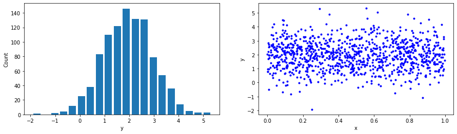
import numpy as npThe same as before, we generate some Gaussian data with \(\mu = 2, \sigma = 1\):
def generate_gaussian_data(m, s, n=1000):
    x = tf.random.uniform(shape=(n,))
    y = tf.random.normal(shape=(len(x),), mean=m, stddev=s)
    return x, y

# Generate normally distributed data with mean = 2 and std dev = 1
x_train, y_train = generate_gaussian_data(m=2, s=1)

plt.figure(figsize=(15, 4))
plt.subplot(1, 2, 1)
plt.hist(y_train, bins=20, rwidth=0.8)
plt.xlabel('y')
plt.ylabel('Count')

plt.subplot(1, 2, 2)
plt.plot(x_train, y_train, 'b.')
plt.xlabel('x')
plt.ylabel('y');
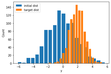
We now use a tensorflow_probability.Normal distribution, with trainable parameters for loc and scale. We do assign some random values to them, which will be updated during the training loop. The initial values we give are purposely off to test whether the gradient descent optimizer will converge. Also, notice how the two distributions (ground truth vs. predicted with random parameters) are misaligned.
# Instantiate a normal distribution with trainable parameters for loc and scale.
# The initial values we assign will be updated during the training process.
normal_dist = tfd.Normal(loc=tf.Variable(0., name='loc'),
                         scale=tf.Variable(2., name='scale'))

plt.hist(normal_dist.sample(1000), bins=20, rwidth=0.8, label='initial dist')
plt.hist(y_train, bins=20, rwidth=0.8, label='target dist')
plt.legend(loc="upper left")
plt.xlabel('y')
plt.ylabel('Count');
def nll(dist, x_train):
"""Calculates the negative log-likelihood for a given distribution
and a data set."""
return -tf.reduce_mean(dist.log_prob(x_train))
@tf.function
def get_loss_and_grads(dist, x_train):
with tf.GradientTape() as tape:
tape.watch(dist.trainable_variables)
loss = nll(dist, x_train)
grads = tape.gradient(loss, dist.trainable_variables)
return loss, grads
# Instantiate a stochastic gradient descent optimizer
optimizer = tf.keras.optimizers.SGD(learning_rate=0.05)
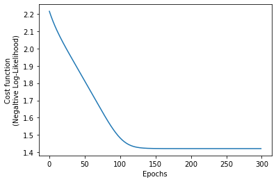
# Custom training loop
epochs = 300
nll_loss = []
for _ in range(epochs):
loss, grads = get_loss_and_grads(normal_dist, y_train)
optimizer.apply_gradients(zip(grads, normal_dist.trainable_variables))
nll_loss.append(loss)
plt.plot(nll_loss)
plt.xlabel('Epochs')
plt.ylabel('Cost function\n(Negaltive Log-Likelihood)');
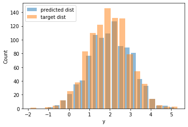
Compare the following figure with the previous one, and see how well-aligned the predicted distribution is with the ground truth distribution.
plt.hist(normal_dist.sample(1000), bins=20, rwidth=0.8, alpha=0.5, label='predicted dist')
plt.hist(y_train, bins=20, rwidth=0.8, alpha=0.5, label='target dist')
plt.legend(loc="upper left")
plt.xlabel('y')
plt.ylabel('Count');
We print the final estimates for the distribution’s parameters, and we see that they are pretty close to the ones we used when we generated our training data.
normal_dist.loc, normal_dist.scale
#    (<tf.Variable 'loc:0' shape=() dtype=float32, numpy=1.9555925>,
#     <tf.Variable 'scale:0' shape=() dtype=float32, numpy=1.0020323>)
Of course, for the normal distribution there exist analytic solutions yielding the optimal parameters. You just assume the log-likelihood:
\[\begin{align*} \log \mathcal{L}(\mu,\sigma^2 \mid x_1,\ldots,x_N) &= \log \prod_{i=1}^N f(x_i) \\ &=\log\left[\left( \frac{1}{\sqrt{2\pi\sigma^2}} \right)^{N} \exp\left( -\frac{ \sum_{i=1}^N (x_i-\mu)^2}{2\sigma^2}\right)\right]\\ &=-\frac{N}{2} \log \left( 2\pi \sigma^2 \right) - \sum_{i=1}^{N} \left( \frac{(x_i - \mu)^2}{2\sigma^2}\right) \end{align*}\]And then solve the following set of equations that maximize log-likelihood (and, therefore, the likelihood):
\[\left\{\frac{\partial \log\mathcal{L}}{\partial \mu}=0, \frac{\partial \log\mathcal{L}}{\partial \sigma}=0\right\}\]I.e., solve for \(\mu, \sigma\) the:
\[\begin{align*} \frac{\partial \log\mathcal{L}}{\partial\mu} &= \sum _{i=1}^n \frac{2 x_i - 2\mu}{2 \sigma^2}=0\\ \frac{\partial \log\mathcal{L}}{\partial\sigma} &=-\frac{N}{\sigma} + \sum_{i=1}^{N} \frac{(x_i-\mu)^2}{\sigma^3}=0 \end{align*}\]The solutions are the mean value and standard deviation of the sample:
\[\begin{align*} \mu_\text{MLE} &= \frac{1}{N} \sum_{i=1}^{N} x_i\\ \sigma_\text{MLE} &= \frac{1}{N} \sum_{i=1}^{N} (x_i - \mu)^2 \end{align*}\]Indeed:
tf.reduce_mean(y_train), tf.math.reduce_std(y_train)

#    (<tf.Tensor: shape=(), dtype=float32, numpy=1.9556075>,
#     <tf.Tensor: shape=(), dtype=float32, numpy=1.0020313>)
However, in most cases, this optimization problem cannot be solved analytically, and therefore we need to attack it numerically.