A simple example of perturbation theory
mathematics perturbation theoryI was looking at the video lectures of Carl Bender on mathematical physics at YouTube. What a great teacher Carl Bender is! The first lectures are an introduction to the perturbation theory. They start with a straightforward problem, where we are asked to find the real root of the following quintic equation:
\[x^5 + x = 1\]This equation cannot be solved exactly, like the quadratic, cubic, or quartic equations. However, the perturbation theory allows us to solve it with arbitrarily high precision. EDIT: Professor Jean Côté kindly corrected me that the equation can be factored as \((x^2-x+1)(x^3+x^2-1) = 0\) which can be solved analytically. Thanks Jean!
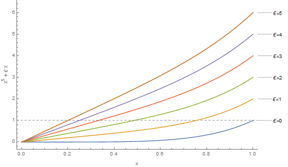
The first step when doing perturbation theory is to introduce the perturbation factor \(\epsilon\) into our problem. This is, to some degree, an art, but the general rule to follow is this. We put \(\epsilon\) into our problem in such a way, that when we set \(\epsilon = 0\), that is when we consider the unperturbed problem, we can solve it exactly. For instance, if we put \(\epsilon\) as \(x^5 + \epsilon x = 1\), then for \(\epsilon = 0\), we get \(x^5 = 1\), that we can solve exactly (\(x = 1\)).
The second step is to assume that the solution to the perturbed problem can be described by an infinite power series of \(\epsilon\):
\[x(\epsilon) = \sum_{n=0}^\infty a_n \epsilon^n\]In this particular example, let us consider only the first 4 terms \(a_0, a_1, a_2, a_3\):
\[x(\epsilon) = a_0 + a_1 \epsilon + a_2 \epsilon^2 + a_3 \epsilon^3 = 1 + a_1 \epsilon + a_2 \epsilon^2 + a_3 \epsilon^3\]Why did we set \(a_0 = 1\)? Well, \(x(0) = a_0\) and we already established that \(x(0) = 1\) when we solved the unperturbed problem. Now, since \(x(\epsilon)\) is a solution to the perturbed problem, then it must satisfy the initial equation that we are solving:
\[x(\epsilon)^5 + \epsilon x(\epsilon) = 1 \Leftrightarrow (1+a_1\epsilon + a_2\epsilon^2 + a_3 \epsilon^3)^5 + \epsilon (1+a_1\epsilon+a_2 \epsilon^2 + a_3 \epsilon^3) = 1\]At this point, I’d probably fire up a Mathematica instance and let it handle the calculations, but Professor Carl Bender proceeded boldly by reminding us of the following identity:
\[(1 + s)^5 = 1 + 5s + 10s^2 + 10 s^3 + \ldots\]And he let \(s = a_1\epsilon + a_2\epsilon^2 + a_3 \epsilon^3\)
Therefore:
\[\begin{align*} &1 + 5a_1\epsilon + 5a_2\epsilon^2 + 5a_3\epsilon^3 + 10(a_1^2\epsilon^2 + 2a_1 a_2 \epsilon^3 + \ldots) + \ldots\\ &=1 + 5a_1\epsilon + \epsilon^2(5a_2+10a_1^2 ) + \epsilon^3(5a_3 + 20a_1 a_2) + \ldots\\ \end{align*}\]We also need to add the expansion of \(\epsilon(1+a_1\epsilon + a_2\epsilon^2 + a_3\epsilon^3)\). Finally, we get:
\[\begin{align*} 1 + 5a_1\epsilon + \epsilon^2(5a_2+10a_1^2 ) + \epsilon^3(5a_3 + 20a_1 a_2) + \ldots\\ \epsilon + a_1 \epsilon^2 + a_2 \epsilon^3 + \ldots = 1 \end{align*}\]In the left hand side we have a polynomial of \(\epsilon\) and in the right hand size we also have a polynomial of \(\epsilon\) where all of its coefficients are zero, except for the constant term which is equal to 1. By invoking the uniqueness of the power series expansion, we require that the terms of the same order are equal one by one:
\[\begin{align*} a_0 &= 1\\ 1 + 5 a_1 = 0 \Rightarrow a_1 &= -\frac{1}{5}\\ a_1 + 5a_2 + 10a_1^2 = 0 \Rightarrow a_2 = \frac{1}{5} \left[-10\left(-\frac{1}{5}\right)^2 - \left(-\frac{1}{5}\right)\right] \Rightarrow a_2 &= -\frac{1}{25} \end{align*}\]Similarly, we get \(a_3 = -\frac{1}{125}\). Therefore:
\[x(\epsilon) = 1 + a_1 \epsilon + a_2 \epsilon^2 + a_3 \epsilon^3 = 1 - \frac{\epsilon}{5} - \frac{\epsilon^2}{25} - \frac{\epsilon^3}{125}\]So, instead of solving one hard problem, \(x^5 + x = 1\), we solved infinite many hard problems, \(x^5 + \epsilon x = 1\). The final step involves setting \(\epsilon = 1\) in order to extract the solution to our particular problem:
\[x = x(1) = 1 - \frac{1}{5} - \frac{1}{25} -\frac{1}{125} = 0.752\]The precise solution is \(x = 0.754878\). So, with just a couple of terms, we made a pretty good approximation!
You can play with the following Mathematica code:
ClearAll["Global`*"];
f[x_] := x^5 + e*x
vars = {a, b, c};
ans[e_] = 1 + Sum[vars[[k]]*e^k, {k, 1, Length@vars}];
expanded = f[ans[e]] // Expand;
getCoeff[n_] := CoefficientList[expanded, e][[n]]
sols = Table[getCoeff[k] == 0, {k, 2, Length@vars + 1}] // Solve;
f[e_] = ans[e] //. Flatten@sols
For instance, you could add some more terms in the power series expansion by modifying the list of variables withvars = {a,b,c,p,q,r} and get:
Which gives \(x = x(1) = 0.754342\).
By the way, I’ve stumbled upon the formula for the general term \(a_n\):
\[a_n = -\frac{\Gamma\left[(4n-1)/5\right]}{5\Gamma\left[(4-n)/5\right] \Gamma(n+1)}\]ClearAll["Global`*"];
an[n_] := -(Gamma[(4 n - 1)/5]/(5 Gamma[(4 - n)/5]*Gamma[n+1]));
Table[an[n], {n, 0, 10}] // FullSimplifyAnd the result is:
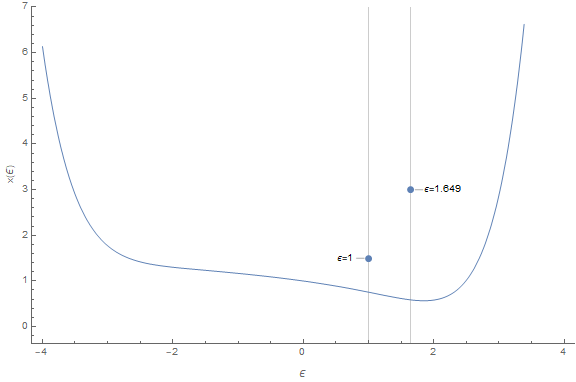
\[\left\{1,-\frac{1}{5},-\frac{1}{25},-\frac{1}{125},0,\frac{21}{15625},\frac{78}{78125},\frac{187}{390625},\frac{286}{1953125},0,-\frac{9367}{244140625}\right\}\]I wasn’t able to calculate the radius of convergence, but my book says that it’s \(R = 5/4^{4/5} = 1.64938\). Therefore, \(\epsilon = 1\) is inside the radius. Here you can see the value of \(x(\epsilon)\) for various values of \(\epsilon\) and notice how it blows up for \(\epsilon > R\).
Naturally, one could ask “Why not put the \(\epsilon\) parameter in front of \(x^5\) in the equation \(x^5 + x = 1\)” ? That is, why not write \(\epsilon x^5 + x = 1\). It turns out that if you do that, the answer \(x(\epsilon)\) you get is a divergent series. However, this is when things start to get very interesting. Because, contrary to what I knew until know and contrary to my intuition, a divergent series may contain valuable information that can be extracted by rewriting it in such a way that it converges.