How to sum a divergent series with Pade approximation
mathematics perturbation theorySo, this is a follow-up post on my previous post where we used perturbation theory to calculate the real root of \(x^5 + x = 1\). In today’s post, we will, again, use perturbation theory to solve the same problem, but this time we will introduce the \(\epsilon\) factor in front of \(x^5\). Concretely, we will try to solve:
\[\epsilon x^5 + x = 1\]This change might seem innocuous at first sight, but it turns out very “violent” because by letting \(\epsilon = 0\), we vanish the term \(x^5\) and, therefore, the other 4 complex roots of the equation. This intervention drastically changes the underlying structure of the problem, and you shall see how it will complicate things later on. Instead of doing the calculations by hand, we will indulge ourselves with Mathematica this time.
ClearAll["Global`*"];
(* Note how epsilon factor is in front of x^5 *)
f[x_] := e*x^5 + x
vars = {a, b, c, r, s, t, u, v};
ans[e_] = 1 + Sum[vars[[k]]*e^k, {k, 1, Length@vars}];
expanded = f[ans[e]] // Expand;
getCoeff[n_] := CoefficientList[expanded, e][[n]]
sols = Table[getCoeff[k] == 0, {k, 2, Length@vars + 1}] // Solve;
f[e_] = ans[e] //. Flatten@sols
By running the code above, we get the following power series representation of the answer \(x(\epsilon)\):
\[x(\epsilon) = 1 - e + 5 e^2 - 35 e^3 + 285 e^4 -2530 e^5 + 23751 e^6 -231880 e^7 + 2330445 e^8\]However, if we proceed like before and set \(\epsilon = 1\) to retrieve the answer to our particular problem, we get a result that is way off:
\[x(1) = 2120041\]Adding more terms to the series won’t help as the sums will continue to diverge. How can we penetrate this barrier, if at all? Enter Padé approximation. I won’t go into much detail, but the idea is to rewrite \(x(\epsilon)\) as a ratio of two polynomials. In the general case we have a power series:
\[A(x) = \sum_{n=0}^\infty a_n x^n\]Even if \(A(x)\) is divergent, it may still be possible to approximate \(A(x)\) with a ratio of two polynomials, \(P_L(x)\) and \(Q_M(x)\), of degree \(L\) and \(M\), respectively. I’ll let this sink for a moment. Even if a power series \(A(x)\) diverges, its coefficients \(a_n\) contain information on how to rewrite \(A(x)\) in a way that it converges. How awesome is that?! Without loss of generality we let \(q_0 = 1\) and, therefore:
\[A(x) = \frac{P_L(x)}{Q_M(x)} = \frac{\sum_\limits{n=0}^{L}p_n x^n}{1 + \sum_\limits{n=1}^{M}q_n x^n}\]So, all we have to do is to determine the \(L + M + 1\) coefficients of the polynomials \(P_L\) and \(Q_M\), i.e. to determine the coefficients \(p_0, p_1, p_2, \ldots, p_L\) and \(q_1, q_2, \ldots, q_M\) (recall that we let \(q_0 = 1\)):
\[A(x) Q_M(x) - P_L(x) = 0\]If we expand \(A(x), Q_M(x), P_L(x)\) we get:
\[\underbrace{\left(a_0 + a_1 x + a_2 x^2 + \ldots \right)}_{A(x)} \underbrace{(1 + q_1 x + q_2 x^2 + \ldots + q_M x^M)}_{Q_M(x)} - \underbrace{(p_0 + p_1 x + p_2 x^2 + \ldots + p_L x^L)}_{P_L(x)} = 0\]If we gather the coefficients and require them to be zero, we get a system of linear equations:
\[\begin{align*} a_0-p_0 &= 0 \\ a_0 q_1+a_1-p_1 &= 0 \\ a_1 q_1+a_0 q_2+a_2-p_2 &= 0\\ a_2 q_1+a_1 q_2+a_0 q_3+a_3-p_3 &= 0\\ \vdots \end{align*}\]The \(a_0, a_1, a_2, \ldots\) are known. They are the coefficients of the divergent series \(A(x)\) that we want to re-express in a form that converges. Let’s see how this goes in our example.
P[m_, x_] := Sum[Subscript[p, j]*x^j, {j, 0, m}]
Q[n_, x_] := 1 + Sum[Subscript[q, j]*x^j, {j, 1, n}]
R[m_, n_, x_] := P[m, x]/Q[n, x]
A[n_, x_] := Sum[Subscript[a, j]*x^j, {j, 0, n}]
getACoeff[n_] := CoefficientList[f[e], e][[n]]
as = Table[Subscript[a, n - 1] -> getACoeff[n], {n, 1, Length@CoefficientList[f[x], x]}]
lhs[n_] := CoefficientList[A[Length@as, x] * Q[n, x] - P[n, x] // Expand, x]
deg = 4;
sol = Table[lhs[deg][[n]] == 0 /. as, {n, 1, 2*deg + 1}] // NSolve
padeApprox[x_] = R[deg, deg, x] /. sol[[1]]Finally, we set \(\epsilon = 1\) and we get:
\[x(1) = 0.757789\]Which is pretty close to the precise solution \(x=0.754878\), corresponding to a relative error about \(0.4\%\). That’s quite an improvement over our first attempt that yielded \(x(1) = 2120041\).
Padé approximation of the exponential function
Let’s, for the fun of it, calculate the Padé approximation of the exponential function \(\text{exp}(x)\). First, we need to write \(\text{exp}(x)\) as a power series \(A(x)\).
exps = Series[Exp[x], {x, 0, 20}];
getACoeff[n_] := CoefficientList[exps, x][[n]]
as = Table[Subscript[a, n - 1] -> getACoeff[n], {n, 1, Length@CoefficientList[exps, x]}]
The code above gives the coefficients of the Taylor series expansion of the exponential function. Mind that the Taylor series is convergent, but we will approximate it with Padé nonetheless:
\[\left\{a_0\to 1,a_1\to 1,a_2\to \frac{1}{2},a_3\to \frac{1}{6},a_4\to \frac{1}{24},a_5\to \frac{1}{120},a_6\to \frac{1}{720},a_7\to \frac{1}{5040},a_8\to \frac{1}{40320},\ldots\right\}\]lhs[n_] := CoefficientList[A[Length@as, x]*Q[n, x] - P[n, x] // Expand, x]
deg = 3;
sol = Table[lhs[deg][[n]] == 0 /. as, {n, 1, 2*deg + 1}] // SolveThe solution to the system provides us with the coefficients of polynomials \(P_3(x)\) and \(Q_3(x)\):
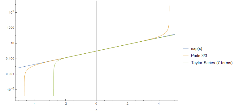
\[\text{exp}(x) = \frac{1 + \frac{x}{2} + \frac{x^2}{10} + \frac{x^3}{120}}{1-\frac{x}{2}+\frac{x^2}{10}-\frac{x^3}{120}}\]Here we plot the value of \(\text{exp}(x)\) along with the Padé \(3/3\) approximation vs. a Taylor series with 7 terms.