Bayesian connection to LASSO and ridge regression
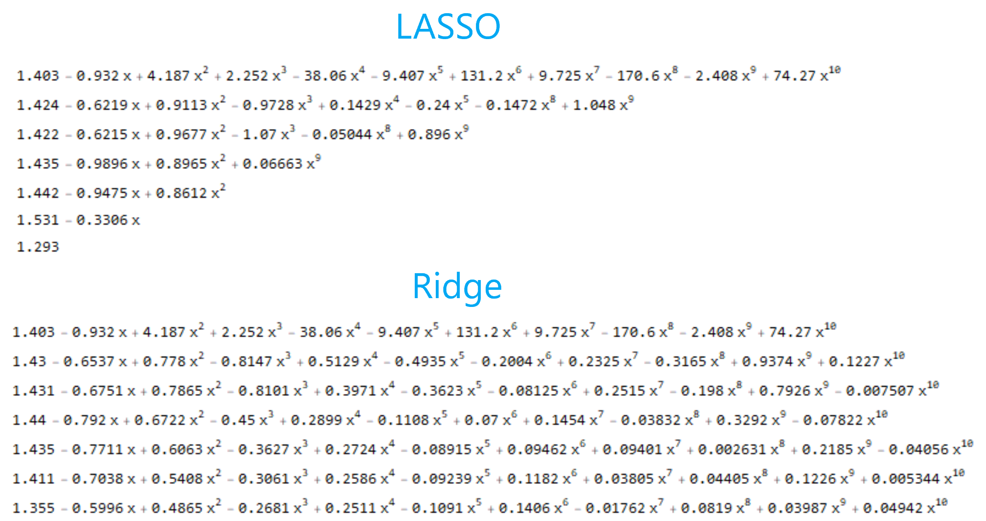
Bayes theorem machine learning mathematics statisticsSo, I was reading “An Introduction to Statistical Learning with Applications in R”, which by the way, is freely available here. On page 227 the authors provide a Bayesian point of view to both ridge and LASSO regression. We have already discussed in a previous post, how LASSO regularization invokes sparsity by driving some of the model’s parameters to become zero, for increasing values of \(\lambda\). As opposed to ridge regression, which keeps every parameter of the model small without forcing it to become precisely zero. Here is a list of regression models, fitted on the same data points, as a function of increasing \(\lambda\):
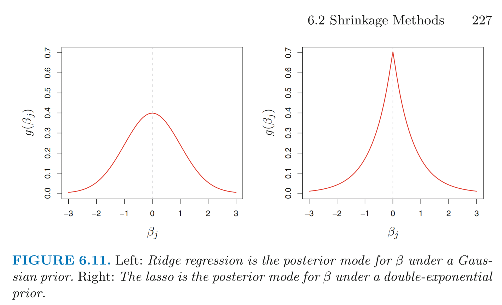
To approach the issue from a Bayesian standpoint, we will assume the usual linear model with normal errors and combine it with a specific prior distribution for the parameters \(\beta\). For ridge regression, the prior is a Gaussian with mean zero and standard deviation a function of \(\lambda\), whereas, for LASSO, the distribution is a double-exponential (also known as Laplace distribution) with mean zero and a scale parameter a function of \(\lambda\). As you can see in the following image, taken from the book of Gareth James et al., for LASSO, the prior distribution peaks at zero, therefore LASSO expects (a priori) many of the coefficients \(\beta\) to be exactly equal to zero. On the other hand, for ridge regression, the prior distribution is flatter at zero. Therefore it expects coefficients to be normally distributed around zero.
In the book, the mathematical proof is left as an exercise on page 262. We shall solve this exercise and establish the connection between the Bayesian point of view and the two regularization techniques. Here it comes!
(a) Suppose that \(y_i = \beta_0 + \sum_{j=1}^{p}\beta_j x_{ij} + \epsilon_i\), where \(\epsilon_i \sim \mathcal{N}(0, \sigma^2)\). Write out the likelihood for the data.
The likelihood for the data is:
\[\mathcal{L}(Y|X,\beta) = \prod_{i=1}^{n} \frac{1}{\sqrt{2\pi}\sigma}\exp\left(-\frac{\epsilon_i^2}{2\sigma^2}\right) = \left(\frac{1}{\sqrt{2\pi}\sigma}\right)^n \exp\left(-\frac{1}{2\sigma^2}\sum_{i=1}^n\epsilon_i^2\right)\](b) Assume the following prior for \(\beta: \beta_1, \beta_2, \ldots, \beta_p\) are i.i.d. according to a double-exponential distribution with mean 0 and common scale parameter according to a double-exponential distribution with mean 0 and common scale parameter \(\beta\): i.e., \(p(\beta) = (1/2b)\exp(-|\beta|/b)\). Write out the posterior for \(\beta\) in this setting.
Multiplying the prior distribution with the likelihood we get the posterior distribution, up to a proporionality constant:
\[p(\beta|X,Y) \propto \mathcal{L}(Y|X,\beta) p(\beta|X) = \mathcal{L}(Y|X,\beta) p(\beta)\]Substituting we get:
\[\mathcal{L}(Y|X,\beta) p(\beta) = \left(\frac{1}{\sqrt{2\pi}\sigma}\right)^n \exp\left(-\frac{1}{2\sigma^2}\sum_{i=1}^n\epsilon_i^2\right) \left[\frac{1}{2b}\exp\left(-\frac{|\beta|}{b} \right)\right]\](c) Argue that the LASSO estimate is the mode for \(\beta\) under the posterior distribution.
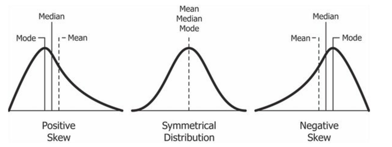
In statistics, the mode of a set of numbers is the number that appears most often. For instance, in the set \(S = \{1, 99, 5, 7, 5, 2, 0\}\) the mode is 5, because 5 appears twice in the set and all the other numbers once. This concept can be extended to continuous values as well. In a normal distribution mean, median and mode coincide. However, in skewed distributions they are different.
Anyway, to show that LASSO estimate is the mode for \(\beta\) under the posterior distribution, we need to show that the most likely value for \(\beta\) is given when the LASSO solution is fulfilled. Here is how we do that. First, we rearrange the expression a bit:
\[\begin{align*} \mathcal{L}(Y|X,\beta) p(\beta) &= \left(\frac{1}{\sqrt{2\pi}\sigma}\right)^n \exp\left(-\frac{1}{2\sigma^2}\sum_{i=1}^n\epsilon_i^2\right) \left[\frac{1}{2b}\exp\left(-\frac{|\beta|}{b} \right)\right]\\ &=\left(\frac{1}{\sqrt{2\pi}\sigma}\right)^n \left(\frac{1}{2b}\right)\exp\left(-\frac{1}{2\sigma^2}\sum_{i=1}^n\epsilon_i^2 - \frac{|\beta|}{b}\right) \end{align*}\]Then we take the logarithm of the product, to simplify the expression (it doesn’t matter if you maximize something or the \(log\) of something):
\[\ln\left[\left(\frac{1}{\sqrt{2\pi}\sigma}\right)^n \left(\frac{1}{2b}\right)\right] -\left(\frac{1}{2\sigma^2}\sum_{i=1}^n\epsilon_i^2 + \frac{|\beta|}{b}\right)\]Therefore, our goal can be formulated as this:
\[\underset{\beta}{\text{maximize}} \left\{ \ln\left[\left(\frac{1}{\sqrt{2\pi}\sigma}\right)^n \left(\frac{1}{2b}\right)\right] -\left(\frac{1}{2\sigma^2}\sum_{i=1}^n\epsilon_i^2 + \frac{|\beta|}{b}\right) \right\}\]But notice that:
\[\underbrace{\left\{ \ln\left[\left(\frac{1}{\sqrt{2\pi}\sigma}\right)^n \left(\frac{1}{2b}\right)\right] - \underbrace{\left(\frac{1}{2\sigma^2}\sum_{i=1}^n\epsilon_i^2 + \frac{|\beta|}{b}\right)}_{\text{Minimize this}} \right\}}_\text{In order to maximize this}\]Therefore:
\[\begin{align*} &\arg \min_\beta \left(\frac{1}{2\sigma^2}\sum_{i=1}^n\epsilon_i^2 + \frac{|\beta|}{b}\right) = \arg \min_\beta \left(\frac{1}{2\sigma^2}\sum_{i=1}^n\epsilon_i^2 + \frac{1}{b}\sum_{j=1}^{p}|\beta_j|\right) =\\ &\arg \min_\beta \frac{1}{2\sigma^2}\left(\sum_{i=1}^n\epsilon_i^2 + \frac{2\sigma^2}{b}\sum_{j=1}^{p}|\beta_j|\right) = \arg \min_\beta \left(\sum_{i=1}^n\epsilon_i^2 + \lambda\sum_{j=1}^{p}|\beta_j|\right) =\\ &\arg \min_\beta \left(\text{RSS} + \lambda\sum_{j=1}^{p}|\beta_j| \right) \end{align*}\]But that is precisely the optimization problem of LASSO, with \(\lambda = \frac{2\sigma^2}{b}\). Recall how in least squares we choose \(\beta_j\) such that we minimize RSS. And then by adding the penalty factor \(\sum_{j=1}^p \vert \beta_j \vert\) we gοt LASSO regression. Therefore, by solving the LASSO optimization problem, we get such values for \(\beta\) that maximize the posterior distribution.
(d) Now assume the following prior for \(\beta: \beta_1,\ldots,\beta_p\) are i.i.d. according to a normal distribution with mean zero and variance \(c\). Write out the posterior for \(\beta\) in this setting.
Same as before, by multiplying the prior distribution with the likelihood we get the posterior distribution, up to a proporionality constant:
\[p(\beta|X,Y) \propto \mathcal{L}(Y|X,\beta) p(\beta|X) = \mathcal{L}(Y|X,\beta) p(\beta)\]Therefore, we first need to calculate \(p(\beta)\):
\[p(\beta) = \prod_{i=1}^p p(\beta_i) = \prod_{i=1}^p \frac{1}{\sqrt{2\pi c}} \exp\left(-\frac{\beta_i^2}{2c}\right) = \left( \frac{1}{\sqrt{2\pi c}} \right)^p \exp\left(-\frac{1}{2c} \sum_{i=1}^p \beta_i^2\right)\]Then, the posterior for \(\beta\) in this setting is:
\[\begin{align*} \mathcal{L}(Y|X,\beta) p(\beta) &= \left(\frac{1}{\sqrt{2\pi}\sigma}\right)^n \exp\left(-\frac{1}{2\sigma^2}\sum_{i=1}^n\epsilon_i^2\right) \left( \frac{1}{\sqrt{2\pi c}} \right)^p \exp\left(-\frac{1}{2c} \sum_{i=1}^p \beta_i^2\right)\\ &=\left(\frac{1}{\sqrt{2\pi}\sigma}\right)^n \left( \frac{1}{\sqrt{2\pi c}} \right)^p \exp\left(-\frac{1}{2\sigma^2}\sum_{i=1}^n\epsilon_i^2 -\frac{1}{2c}\sum_{i=1}^p \beta_i^2\right) \end{align*}\](e) Argue that the ridge regression estimate is both the mode and the mean for \(\beta\) under this posterior distribution.
By the same logic, as before, first we take the logarithm:
\[\begin{align*} &\ln\left[\left(\frac{1}{\sqrt{2\pi}\sigma}\right)^n \left( \frac{1}{\sqrt{2\pi c}} \right)^p \right] -\left(\frac{1}{2\sigma^2}\sum_{i=1}^n\epsilon_i^2 + \frac{1}{2c}\sum_{i=1}^p \beta_i^2\right) \end{align*}\]Then, we recall that to show that rigdge estimate is the mode for \(\beta\) under the posterior distribution, we need to show that the most likely value for \(\beta\) is given by that solution of the ridge optimization problem:
\[\begin{align*} &\arg\min_\beta \left(\frac{1}{2\sigma^2}\sum_{i=1}^n\epsilon_i^2 + \frac{1}{2c}\sum_{i=1}^p \beta_i^2\right) = \arg\min_\beta \frac{1}{2\sigma^2} \left(\sum_{i=1}^n\epsilon_i^2 + \frac{2\sigma^2}{2c}\sum_{i=1}^p \beta_i^2\right) =\\ &\arg\min_\beta \left(\sum_{i=1}^n\epsilon_i^2 + \lambda\sum_{i=1}^p \beta_i^2\right) = \arg\min_\beta \left(\text{RSS} + \lambda\sum_{i=1}^p \beta_i^2\right) \end{align*}\]But that is precisely the formulation of ridge optimization, with \(\lambda = \frac{\sigma^2}{c}\). Recall how in least squares we choose \(\beta_j\) such that we minimize RSS. And then by adding the penalty factor \(\sum_{j=1}^p \vert \beta_j \vert^2\) we gοt ridge regression.