Alternating direction method of multipliers and Robust PCA

Contents

• What’s wrong with vanilla PCA?
• Problem formulation
• When is \(\mathbf{X} = \mathbf{L} + \mathbf{S}\) separation meaningful?
• Applications of Robust PCA
• Augmented Lagrangian method
• Example code in Mathematica
• References

What’s wrong with vanilla PCA?

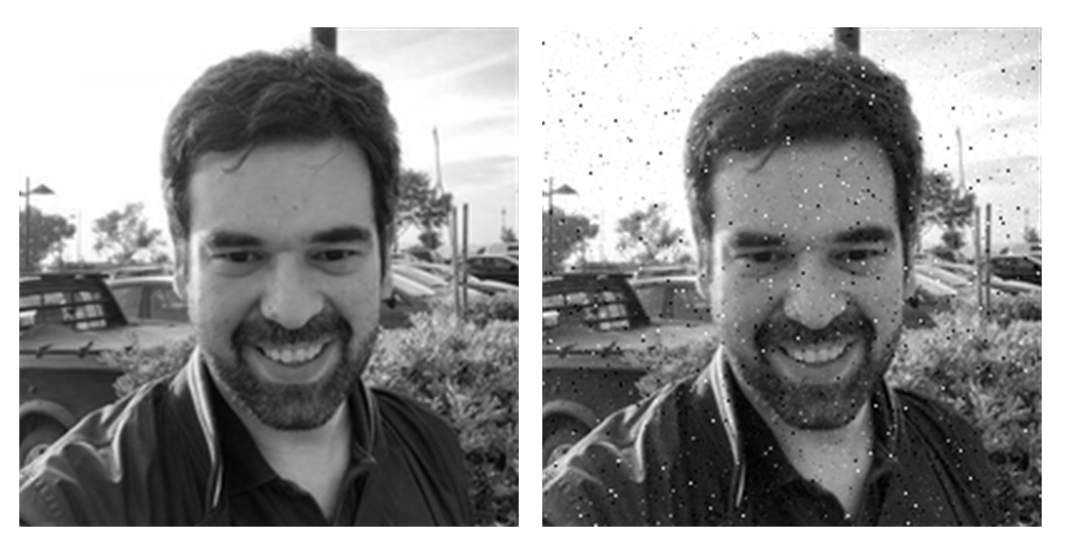
In the previous blog post, we discussed some of the limitations of principle component analysis. One such restriction arises when there exist gross errors, corruption in the data, even just outliers. A method to handle such cases is the so-called “Robust PCA”, which we will talk about today. To understand what’s wrong with regular PCA, take a look at the following two images. The original image is on the left, whereas on the right we added some salt-and-pepper noise.

origImg =
 ColorConvert[
  ImageResize[Import["C:\\Users\\stathis\\Desktop\\me.jpg"], 200], "Grayscale"]

corruptedImg = ImageAdd[
  origImg, 
  RandomImage[CauchyDistribution[0, 0.005], ImageDimensions@origImg]]

Style[Grid[{{origImg, corruptedImg}}], ImageSizeMultipliers -> 1]

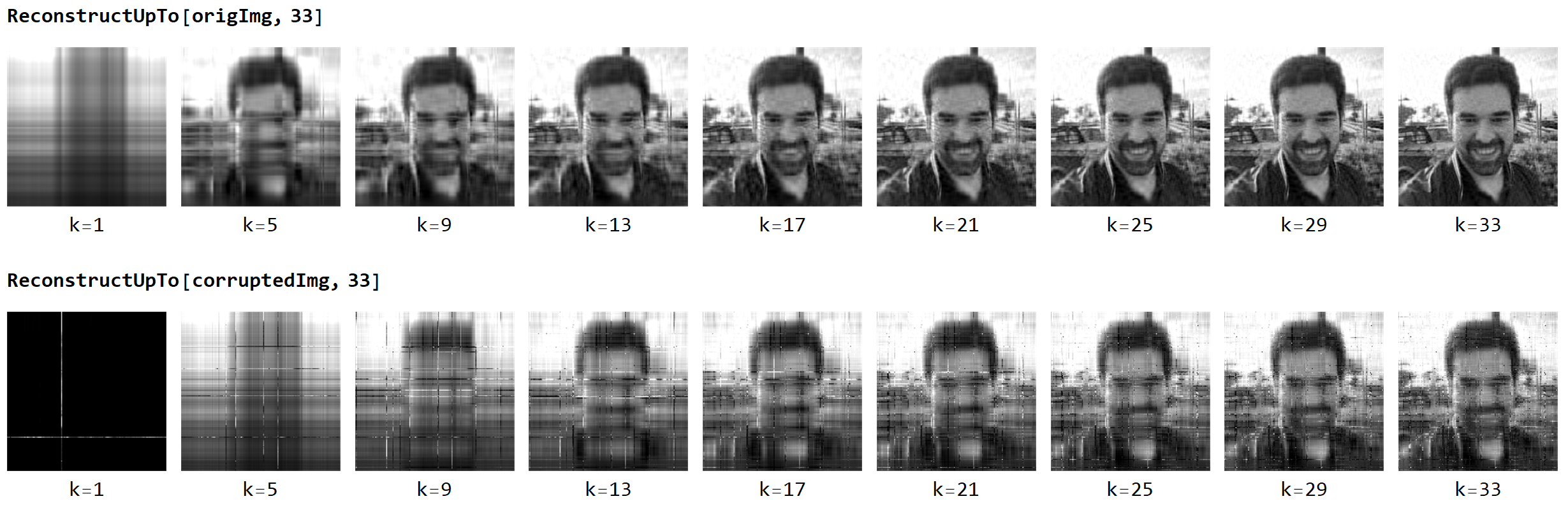
Let’s see what happens if we perform an SVD and then try to reconstruct the two images:

Reconstruct[svd_, k_] := 
 Labeled[Image[svd[[1]] . svd[[2]] . Transpose[svd[[3]]]], 
  "k=" <> ToString@k]

ReconstructUpTo[img_, k_] :=
 Grid[{Table[
    With[{svd = SingularValueDecomposition[ImageData@img, i]},
     Reconstruct[svd, i]], {i, 1, k, 4}]
   }]

As you may notice, the decomposition of the corrupted image is way worse compared to the original one (for the same number of singular values). The presence of a handful of outlier values is enough to derail the reconstruction. We used SVD here, but essentially it’s the same for PCA (we will talk in a future post on the connection between PCA and SVD).

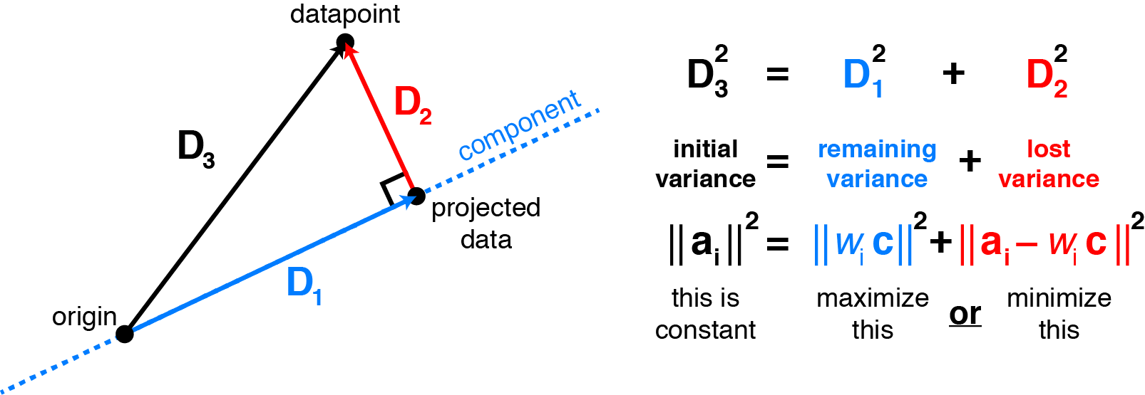
If you want to dig in a bit deeper on why this happens, consider that PCA is a low-rank approximation of the data that minimizes the residuals’ Frobenius norm. In this sense, its vulnerability to outliers is similar to the vulnerability of least-squares to outliers. Due to the squaring of deviations from the outliers, they dominate the total norm and drive the PCA components. The following image is taken from this fantastic blog post, and provides an intuition on why by maximizing variance, PCA minimizes the least-squares reconstruction error.

Feel free to also check the Eckard-Young theorem.

Problem formulation

Suppose that we are given a large matrix \(\mathbf{X}\in \mathbb{R}^{m,n}\), such that it can be decomposed as a sum of a low-rank matrix \(\mathbf{L}\) and a sparse matrix \(\mathbf{S}\), i.e., \(\mathbf{X} = \mathbf{L} + \mathbf{S}\). If you are unfamiliar with the terms, the rank of a matrix is defined as either the maximum number of linearly independent column vectors in the matrix or, equivalently, as the maximum number of linearly independent row vectors. A sparse matrix contains very few non-zero elements.

       

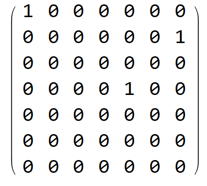
Left: Low-rank matrix. Only the first and the last columns are linearly independent. Right: Sparse matrix. Only three elements are non-zero.

Alright, so our problem is akin to decomposing the image on the left as the sum of the two images on the right:

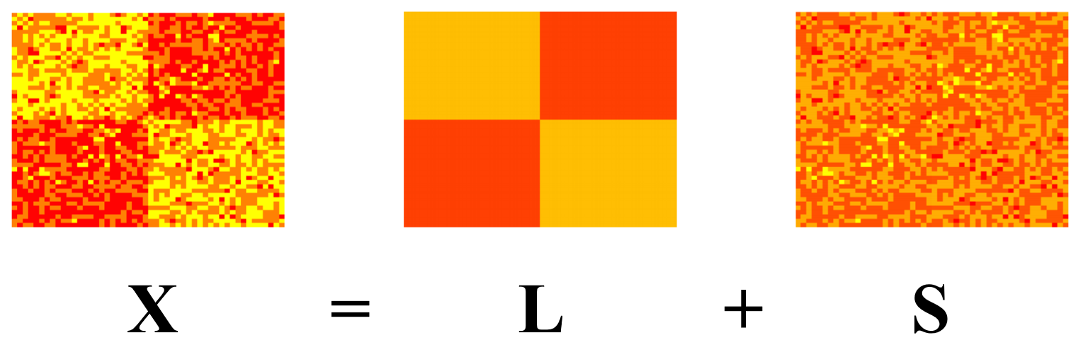
Image taken from a presentation of Yuxin Chen.

In this setup, we do not know the rank of matrix \(\mathbf{L}\), nor the positions of the zeros in the sparse matrix \(\mathbf{S}\) or even how many of them there are. The optimization problem we are called to solve is:

\[\mathop{\mathrm{arg\,min}}_{L,S} \,\,\mathop{\mathrm{rank}}(\mathbf{L}) + \lambda \left\Vert \mathbf{S}\right\Vert_{\infty}, \,\, s.t. \mathbf{X} = \mathbf{L} + \mathbf{S}\]

Where \(\left\Vert \mathbf{S}\right\Vert_\infty\) is the infinity norm that goes down as the non-zero elements of a matrix go down. The parameter \(\lambda\) defines the relative contribution of the two terms in the optimization objective. If we assume a large value for \(\lambda\), then the optimizer will try harder to decrease the density of the matrix \(\mathbf{S}\) to achieve sparseness.

However, the above formulation is literally a disaster in an optimization context. We have twice as many unknown as knowns, the problem has a combinatorial complexity and both terms are non-convex. Since we really like optimizing convex functions, we replace the original problem with a new one, that is “relaxed” in such a way that it now is convex:

\[\mathop{\mathrm{arg\,min}}_{L,S} \,\, \left\Vert \mathbf{L}\right\Vert_* + \lambda \left\Vert \mathbf{S}\right\Vert_1, \,\, s.t. \mathbf{X} = \mathbf{L} + \mathbf{S}\]

Where \(\left\Vert \mathbf{L}\right\Vert_*\) is the nuclear norm of matrix \(\mathbf{L}\), i.e., the sum of \(\mathbf{L}\)’s singular values which is used as a proxy for the rank of the matrix \(\left\Vert \mathbf{L}\right\Vert_* \stackrel{\text{def}}{=} \sum_i \sigma_i(\mathbf{L})\) and \(\left\Vert \mathbf{S}\right\Vert_1\) is the element-wise \(\ell_1\) norm \(\left\Vert \mathbf{S}\right\Vert_1 \stackrel{\text{def}}{=} \sum_{ij} |S_{ij}|\).

When is \(\mathbf{X} = \mathbf{L} + \mathbf{S}\) separation meaningful?

1. When \(\mathbf{L}\) is not sparse, e.g., its singular values are reasonably spread out.
2. When \(\mathbf{S}\) is not low rank, e.g., it does not have all non zero elements in a column or in a few columns.

Otherwise, the decomposition is simply not feasible. For instance, check the following sparse matrices. The left one happens to also be low-rank since only the first column is linear independent! This is a no-go!

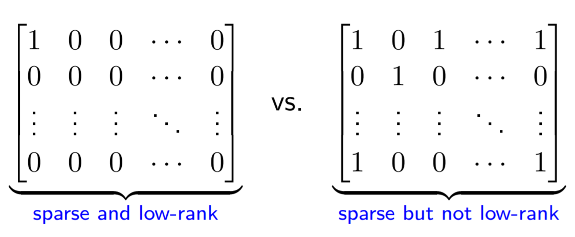
Image taken from a presentation of Yuxin Chen.

Applications of Robust PCA

• Video surveillance. The background variations of a video are modeled as a low-rank matrix, and the foreground objects such as pedestrians and cars are modeled as sparse errors superimposed on the low-rank background. How do we do that? We take every frame and reshape it into a long column vector, and then we use these long column vectors to construct the matrix \(\mathbf{X}\). E.g., in the following case, the video consists of 100 frames.

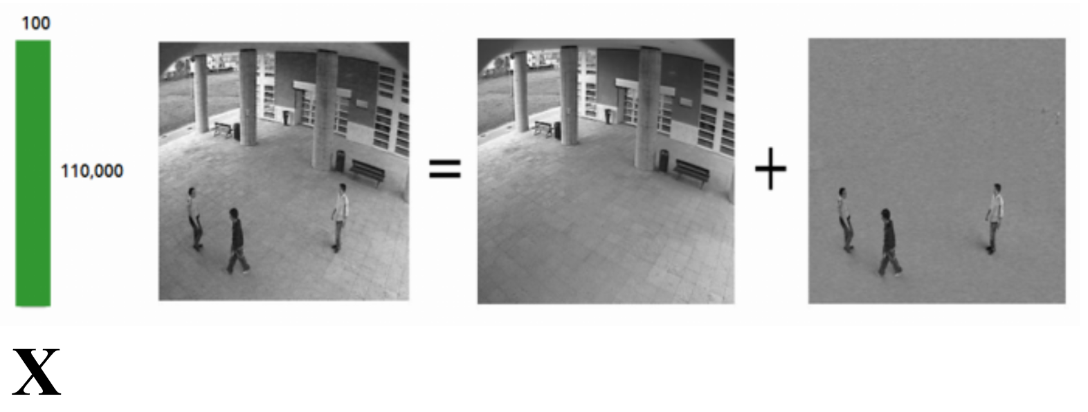
Image taken from here.

• Latent semantic indexing. The basic idea here is to generate a document versus term matrix whose entries reflect a term’s relevance in a document. Then, the decomposing \(\mathbf{X} = \mathbf{L} + \mathbf{S}\), \(\mathbf{L}\) would capture the common words and \(\mathbf{S}\) the few terms that would distinguish the documents.
• Ranking and recommendation systems.
• Face recognition. Removing shadows, specularities, and reflections from facial images.

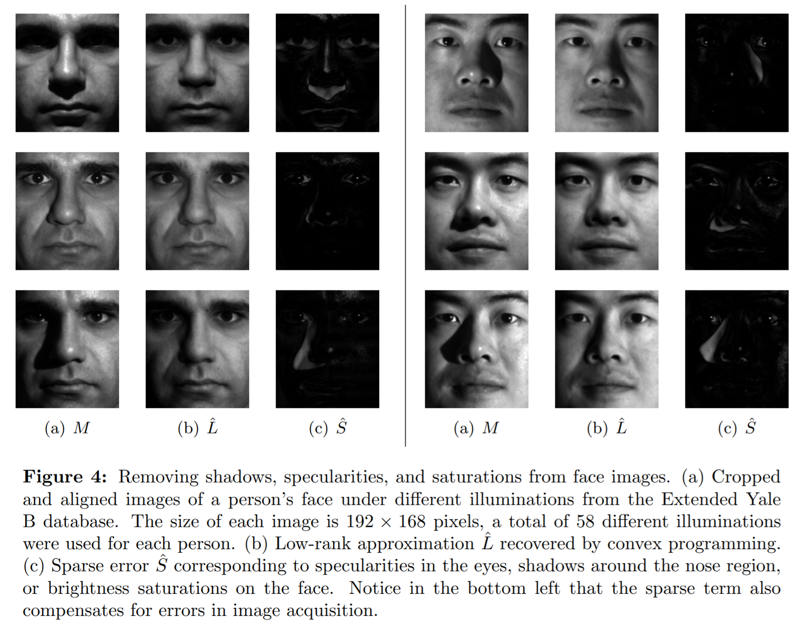
Image taken from here.

Augmented Lagrangian method

The augmented Lagrangian of the optimization problem is:

\[\mathcal{L}(\mathbf{L},\mathbf{S},\mathbf{Y}) = \underbrace{\left\Vert\mathbf{L}\right\Vert _*+ \lambda \left\Vert \mathbf{S}\right\Vert_1 + \left<{\mathbf{Y},\mathbf{X}-\mathbf{L}-\mathbf{S}}\right>}_{\text{Standard Lagrangian}} + \underbrace{\frac{\rho}{2} \left\Vert \mathbf{X} - \mathbf{L} -\mathbf{S}\right\Vert_2^2}_{\text{Augmented Lagrangian term}}\]

Where \(\left<{\mathbf{A},\mathbf{B}}\right>=\text{trace}(\mathbf{A}^*\mathbf{B})\). The quadratic penalty is added to make the objective strongly convex when \(\rho\) is large. This helps convergence without assumptions like strict convexity or even finiteness of the minimized function. Also, the penalty is softer than a barrier, as the iterates are no longer confined to the feasible space. Anyway, a generic ALM algorithm would solve the optimization problem by repeatedly doing the following calculations:

\[(\mathbf{L}_{k+1}, \mathbf{S}_{k+1}) = \mathop{\mathrm{arg\,min}}_{L,S} \,\,\mathcal{L}(\mathbf{L},\mathbf{S},\mathbf{Y}_k)\]

And then updating the Lagrange multipliers:

\[\mathbf{Y}_{k+1}=\underbrace{\mathbf{Y}_k + \rho \underbrace{(\mathbf{X}-\mathbf{L}_{k+1} - \mathbf{S}_{k+1})}_{\text{residual error}}}_{\text{running sum of residual errors}}\]

However, the first step is usually as expensive as solving the initial problem. So we need to do better than this. In the literature, there are dozens of methods designed to solve the problem above. One such method is the so-called Alternating Direction Method of Multipliers. ADMM splits the minimization problem into two smaller and easier to tackle subproblems, where \(\mathbf{L}, \mathbf{S}\) are minimized separately, rather than jointly:

\[\begin{align*} \mathbf{L}_{k+1} &= \mathop{\mathrm{arg\,min}}_{L} \,\,\mathcal{L}(\mathbf{L}, \mathbf{S}_k, \mathbf{Y}_k)\\ \mathbf{S}_{k+1} &= \mathop{\mathrm{arg\,min}}_{S} \,\, \mathcal{L}(\mathbf{L}_{k+1}, \mathbf{S}, \mathbf{Y}_k)\\ \mathbf{Y}_{k+1} &= \mathbf{Y}_k + \rho(\mathbf{X} - \mathbf{L}_{k+1} - \mathbf{S}_{k+1}), \,\,\rho>0 \end{align*}\]

ADMM for solving convex problems globally converges for any penalty parameter \(\rho > 0\) with a sublinear rate \(\mathcal{O}(1/k)\). I listened to Stephen Boyd’s talk on ADMM, and he made the following statement. For every specific optimization problem, a better optimization algorithm than ADMM probably exists. However, as a generic algorithm that can be applied to pretty much every case and give reasonably good results after a few iterations, ADMM is top.

The linear and quadratic terms of the augmented Lagrangian can be combined, by “completing” the square:

\[\begin{align*} \mathbf{L}_{k+1} &= \mathop{\mathrm{arg\,min}}_L \,\, \left\{ \left\Vert\mathbf{L}\right\Vert_* + \frac{\rho}{2}\left\Vert \mathbf{X}_k-\mathbf{L}-\mathbf{S}_k + (1/\rho)\mathbf{Y}_k\right\Vert_2^2\right\}\\ \mathbf{S}_{k+1} &= \mathop{\mathrm{arg\,min}}_S \,\, \left\{ \lambda\left\Vert\mathbf{S}\right\Vert_1 + \frac{\rho}{2}\left\Vert \mathbf{X}_k-\mathbf{L}_{k+1}-\mathbf{S}_k + (1/\rho)\mathbf{Y}_k\right\Vert_2^2\right\}\\ \mathbf{Y}_{k+1} &=\mathbf{Y}_k + \rho\left(\mathbf{X} -\mathbf{L}_{k+1} - \mathbf{S}_{k+1}\right) \end{align*}\]

Sometimes, the transformation \(\mathbf{U}=(1/\rho)\mathbf{Y}\) is used to simplify the expressions above.

This is equivalent to:

\[\begin{aligned} \mathbf{L}_{k+1} &=\mathrm{SVT}_{1/\rho}\left(\mathbf{X}-\mathbf{S}_{k}+\frac{1}{\rho} \mathbf{Y}_{k}\right) \\ \mathbf{S}_{k+1} &=\mathcal{S}_{\lambda/\rho}\left(\mathbf{X}-\mathbf{L}_{k+1}+\frac{1}{\rho} \mathbf{Y}_{k}\right) \\ \mathbf{Y}_{k+1} &=\mathbf{Y}_{k}+\rho\left(\mathbf{X}-\mathbf{L}_{k+1}-\mathbf{S}^{k+1}\right) \end{aligned}\]

Where \(\mathrm{SVT}_{\tau}(\mathbf{X})=\mathbf{U} \mathcal{S}_{\tau}(\mathbf{\Sigma}) \mathbf{V}^{*}\), is the singular value thresholding operator. And \(\mathcal{S}_{\tau}(x)=\operatorname{sgn}(x)\max(\mid x \mid-\tau, 0)\) is the soft thresholding operator.

A remarkable fact is that there is no need for tuning the scalar \(\lambda\) most of the time. There is a universal value that works well, \(\lambda = \frac{1}{\sqrt{\mathrm{max}(m,n)}}\). However, if assumptions are only partially valid, the optimal value of \(\lambda\) may vary slightly. For example, if the matrix \(\mathbf{S}\) is very sparse, we may need to increase \(\lambda\) to recover matrices \(\mathbf{L}\) of larger rank.

Example code in Mathematica

The following code implements the Alternating Direction of Method Multipliers:

(* Define the shrinkage operator aka thresholding operator *)
Shrink[t_, x_] := Sign[x]*Map[Max[#, 0] &, Abs[x] - t, {2}]

RobustPCA[X_] :=
 Module[{m, n, ρ, λ, i, U, Σ, V, L, S, Y, 
   error, tolerance},
  L = ConstantArray[0, Dimensions[X]];
  S = ConstantArray[0, Dimensions[X]];
  Y = ConstantArray[0, Dimensions[X]];
  {m, n} = Dimensions[X];
  ρ = m*n/(4 Norm[X, 1]);
  λ = 1./Sqrt[Max[Dimensions[X]]];
  tolerance = 10^-17*Norm[X, "Frobenius"];
  error = Infinity;
  errors =
   Reap[
    For[i = 1, i <= 10^4 && error > tolerance, i++,
     {U, Σ, V} = 
      SingularValueDecomposition[X - S + (1/ρ)*Y];
     L = U . Shrink[1/ρ, Σ] . Transpose[V];
     S = Shrink[λ /ρ, X - L + (1/ρ)*Y];
     Y = Y + ρ*(X - L - S);
     error = Norm[X - L - S, "Frobenius"];
     Sow[error];
     ]];
  {{L, S}, errors}
]

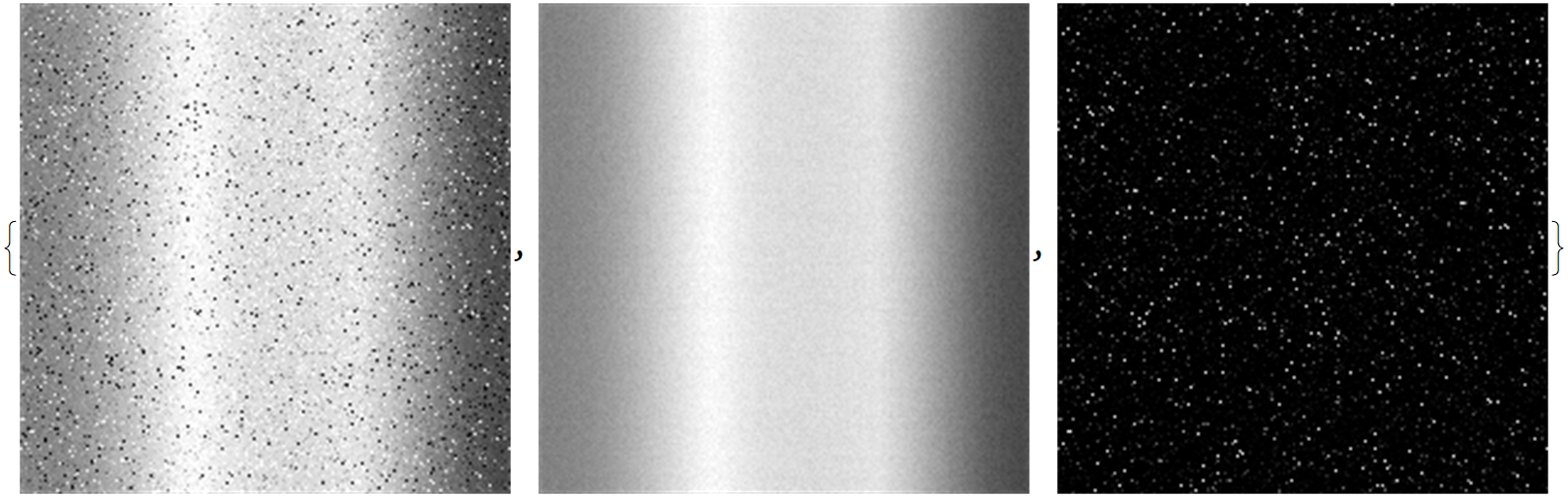
Here is the output of running the above implementation on a rainbow image:

origImg =
 ColorConvert[
  ImageResize[Import["C:\\Users\\stathis\\Desktop\\rainbow.jpg"], 200],
  "Grayscale"]

(* Add some salt-and-pepper noise *)
corruptedImg = ImageAdd[
  origImg, 
  RandomImage[CauchyDistribution[0, 0.02], ImageDimensions@origImg]
  ]
  
X = ImageData[corruptedImg];
{{L, S}, errors} = RobustPCA[X];
Style[Image /@ {X, L, S}, ImageSizeMultipliers -> 1]

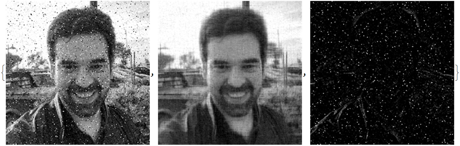
And this is the result of running it on a selfie of mine:

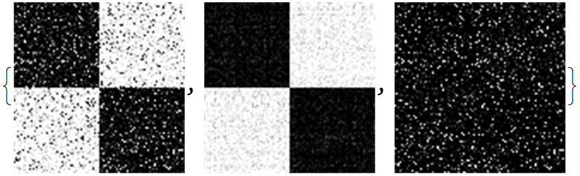
Last, we run the algorithm on a corrupted low-rank image:

Clear[a, b];
a = Join[ConstantArray[0, {50, 50}], ConstantArray[1, {50, 50}]];
b = Reverse[a];
origImg = Image[Join[a, b, 2]]

corruptedImg = ImageAdd[
  origImg, 
  RandomImage[CauchyDistribution[0, 0.1], ImageDimensions@origImg]
  ]

X = ImageData[corruptedImg];
{{L, S}, errors} = RobustPCA[X];
Style[Image /@ {X, L, S}, ImageSizeMultipliers -> 1]

References

1. Candès, EJ et al. Robust principal component analysis? J. ACM 58, 1–37 (2011)
2. Boyd, S et al, Distributed Optimization and Statistical Learning via the Alternating Direction Method of Multipliers.