Principal Component Analysis limitations and how to overcome them
machine learning mathematics statisticsIn the era of big data, our measuring capabilities have exponentially increased. It is often the case that we end up with very high dimensional datasets that we want to “summarize” with low dimensionality projections. PCA is arguably a widely used data dimensionality reduction technique. We have already discussed it in a previous post, where we viewed PCA as a constrained optimization problem solved with Lagrange multipliers. However, there are some limitations of PCA that someone should be familiar with. At the same time, weaknesses in a technique pose opportunities for new developments, as we shall see.
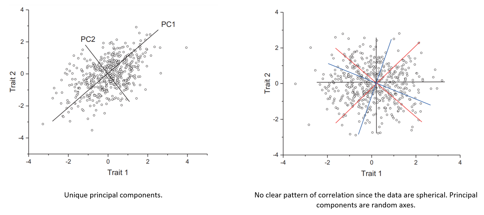
- To apply PCA and produce meaningful results, we must first check whether some assumptions hold, like the presence of linear correlations (e.g., Bartlett’s test of sphericity) or sampling adequacy (e.g., Kaiser-Meyer-Olkin test). This step is often overlooked, and strictly speaking, is not a limitation of PCA but of the person running the analysis. In this context, the principal components must be unique otherwise lack meaning (they are essentially random axes). We already have demonstrated this. Therefore, the distinctiveness of the eigenvalues is a fundamental assumption of PCA that the analyst must test. The following image was taken from here:
- Τhe method relies on linear relationships between the variables in a dataset. So, what if there are correlations but are not linear? There is the so-called called kernel PCA version that allows PCA to also work with non-linear data. Vanilla PCA computes the covariance matrix of the dataset: \(C = \frac{1}{n}\sum_{i=1}^n{\mathbf{x}_i\mathbf{x}_i^\mathsf{T}}\). Kernel PCA, on the other hand, first transforms the data into an even higher-dimensional space where: \(C = \frac{1}{n}\sum_{i=1}^n{\Phi(\mathbf{x}_i)\Phi(\mathbf{x}_i)^\mathsf{T}}\). And only then projects the data onto the eigenvectors of that matrix, just like regular PCA. The kernel trick refers to performing the computation without actually computing \(\Phi(\mathbf{x})\). This is possible only if \(\Phi\) is chosen such that it has a known corresponding kernel. KPCA doesn’t always cut it, so depending on your dataset, you may need to look at other non-linear dimensionality reduction techniques, such as LLE, isomap, or t-SNE.
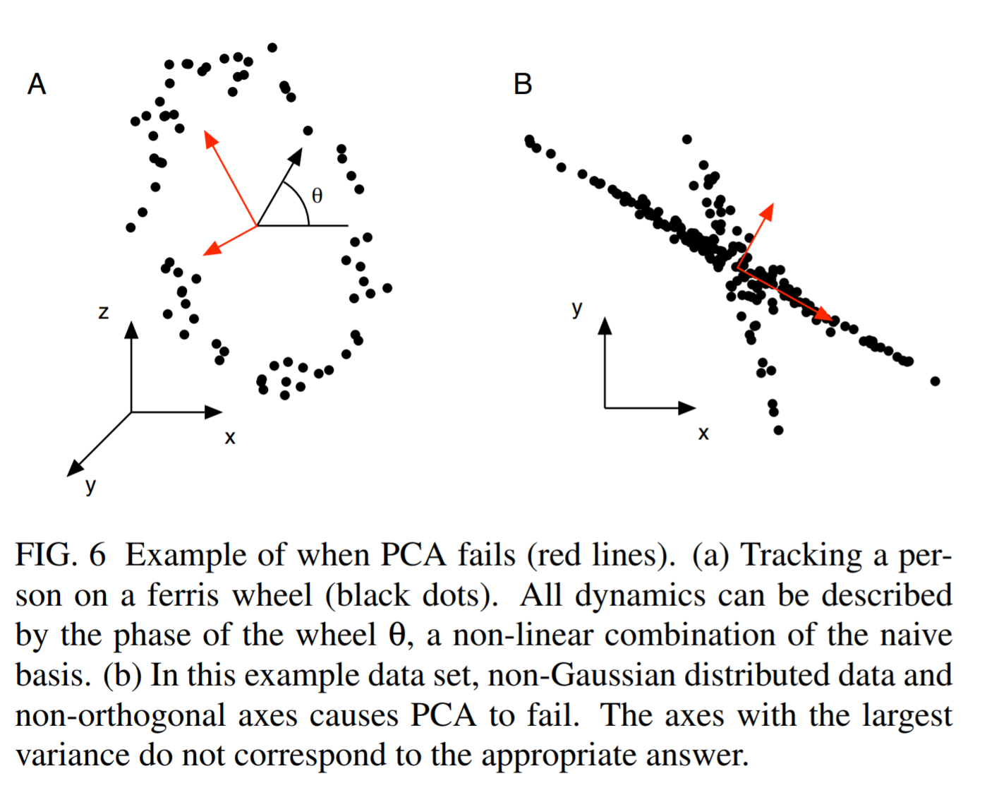
- Another limitation is the assumption of orthogonality, since the principal components are by design orthogonal to each other. Depending on the situation, far “better” basis vectors may exist to summarize the data that are not orthogonal. The following image shows an extreme such case that was taken from here:
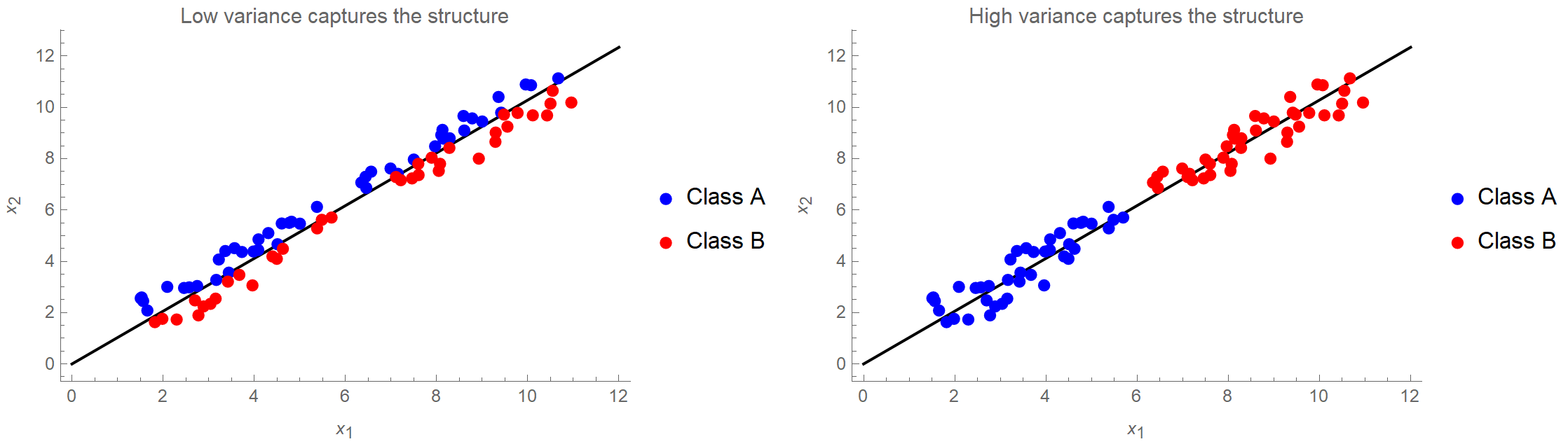
- The next gotcha is that large variance is used as a criterion for the existence of structure in the data. However, sometimes structure is found in places with low variance, as we see in the following image. If we kept only the first principal component, we would be absolutely fine in the right case, but in the left case, we would perform badly in a classification context.
- Next, PCA is scale variant. This means that if the variables in our dataset have different units, some variables will dominate the others simply because they assume bigger values, and therefore contribute more to the overall variance. That’s why we typically transform our data so that they have a unit standard deviation. However, this may or may not be appropriate depending on the research question. E.g., if we are doing PCA on gene expression data, this would put an equal “weight” on each gene. Again, this may or may not be desired. (Also, the data absolutely need to be mean-centered, but I think pretty much everyone is aware of this.)
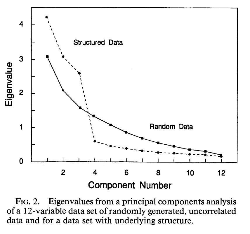
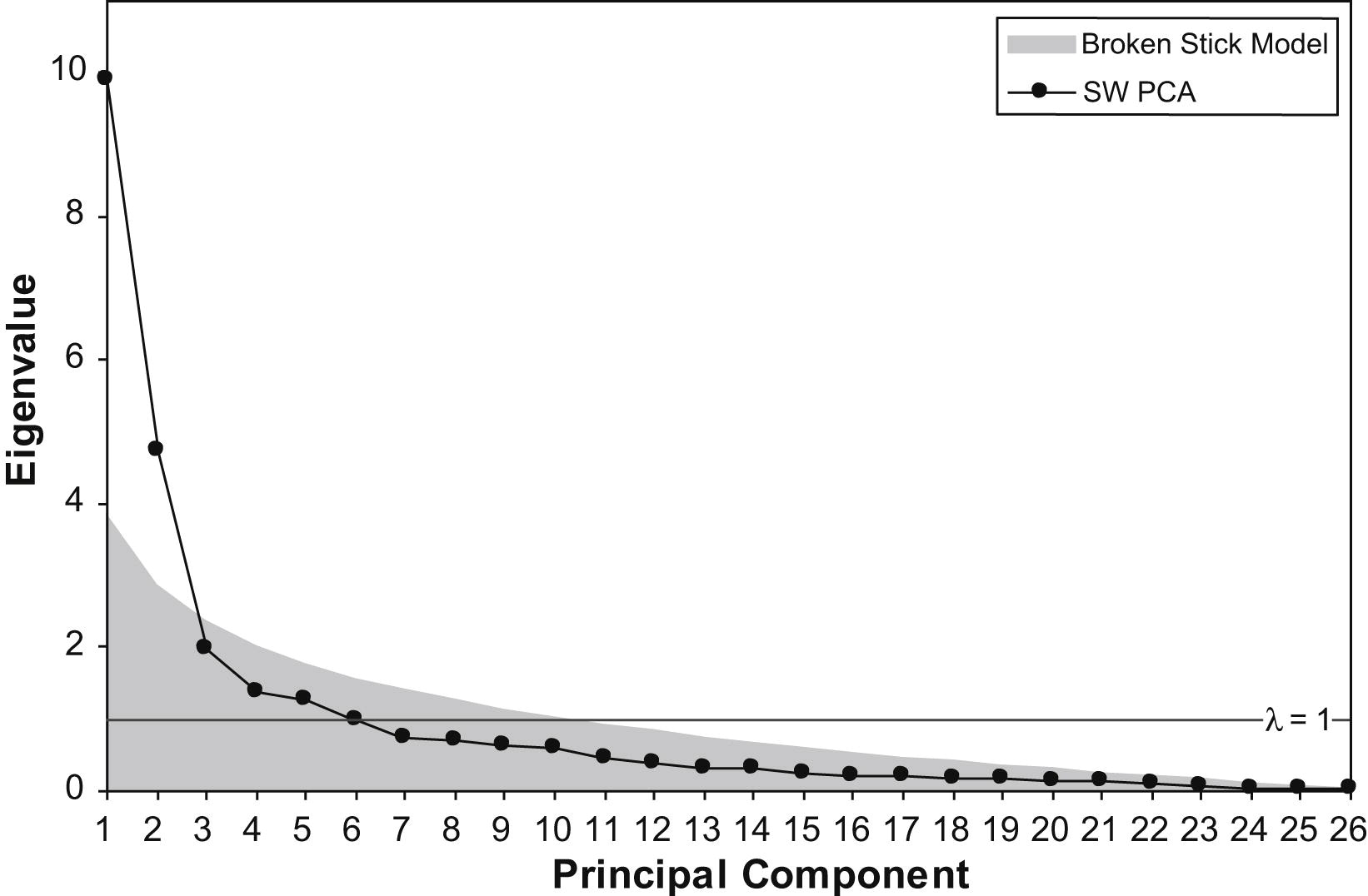
- The point of PCA is to reduce the dimensionality of a dataset. So, how do we decide how many principal components to retain? Approaches often used include visual inspection of the scree plot looking for an “elbow”, keeping components accounting for a fixed amount of the total variance, e.g., 95% of the total variance, or picking components with eigenvalues > 1. However, depending on how robust the analysis needs to be, one should keep in mind that correlations may appear randomly. For instance, the following figure shows the eigenvalues from a PCA of a 12-variable data set of randomly generated, uncorrelated data and for a data set with underlying structure.
Feel free to check the PCDimension R package on how to estimate the number of significant components. One technique is to use the “broken stick” model. The idea behind this is to model \(N\) variances by assuming a stick of unit length and breaking it into \(N\) pieces by randomly (and simultaneously) selecting break points from a uniform distribution. We then compare element-wise the percentage variances of our components against the percentages from the broken stick distribution. As long as observed eigenvalues are higher than the corresponding random broken stick components, we keep the principal components. See for example the following figure where the broken stick model is compared with the eigenvalue > 1 criterion. Another method is to use the bootstrap resampling technique to calculate confidence intervals for the eigenvalues and keep those whose CI contains 1.
- One very important issue is that of interpretability. Once we have replaced our original variables with the principal components, it’s not always entirely trivial to interpret the results.
- Sometimes, depending on the data’s structure and the research question, one might apply a rotation after PCA to simplify the components’ interpretation. Such rotations include Varimax and oblique rotations (however, these have their own set of limitations, e.g., they might produce components that don’t correspond to successive maximal variance or produce components that are correlated or give slightly different results every time they are applied given that they are iterative methods).
- Another path to simplifying PCs, therefore to interpretation, is to force additional constraints on the new variables, e.g., a direct \(L_1\) constraint. Or reformulate PCA as a regression problem and use LASSO, which we already discussed in the context of regularization. Either way, that’s the field of Sparse PCA.
- Last, PCA has a hard time working with missing data and outliers. Here is a review paper on how to impute missing data in the context of PCA. With respect to handling outliers and corrupted data, there is Robust PCA. You may check out a great video on YouTube from Steve Brunton on RPCA, and a hopefully decent blog post I wrote.