The joy of not google'ing: Short to long stick ratio in broken rods
mathematicsIntroduction
Hola! Long time no see! In the past months, I’ve been swamped working as a machine learning engineer at Chronicles Health, a digital health company, on a course to revolutionize the management of inflammatory bowel disease.
But I’m back! However, today’s post won’t cover some fancy machine learning algorithm or data science topic. Instead, let me tell you about a neat little problem I found on the Internet (credits to Gianni Sarcone). It turns out that, like many people, I’ve become extremely good at googling stuff but less so at thinking for myself. So, I decided to solve this cute little puzzle in the traditional “analog” way, with pen and paper, without any online help :) And as a matter of fact, I encourage you to do the same. Once every now and then, try to solve a relatively simple science problem without referencing online resources. If you need some formula or a theorem, look it up in a paper book, seriously. You will be amazed at how beneficial this approach will be to your problem-solving skills.
Problem statement
Suppose that we throw 10.000 rods against a rock, and they break at random places. What is the average ratio of the length of the short piece to the length of the long piece?
Solution
We start by modeling the problem, which probably is the most critical part of a problem-solving process. The way we set it up will largely define the next steps. So, we need to assign symbols to the various involved components. There’s a rod, and two pieces, a short and a long one. Let’s say that the rod has length \(L\). Then, if we agree that the short piece is of size \(x\), the remainder will be the long one with length \(L-x\). Mind that \(x\) is not fixed; it’s a random variable since we have 10.000 rods, and so is \(L-x\).
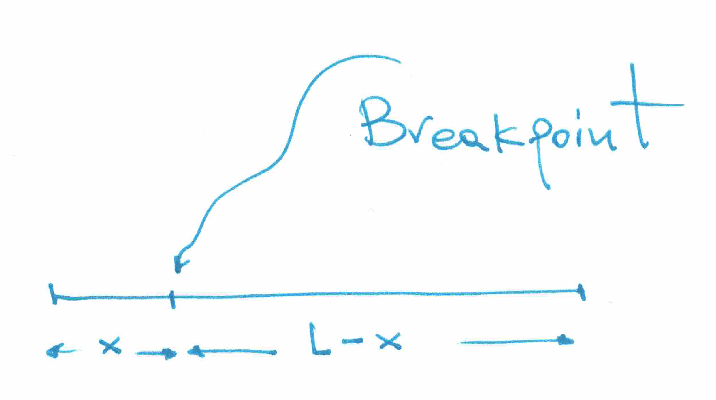
Every time we translate the statement of a problem into mathematical symbols and expressions, we need to constrain the values that our variables assume so that our setup always “makes sense”. Since \(x\) is the short part, it really can’t be larger than a half rod because it would be the long one! So, \(x\in[0,L/2]\). Also, \(L>0\) or there would be any rod, to begin with. So, we are interested in the average ratio of the short to long pieces, i.e.:
\[\text{avg. ratio} = \left<x/(L-x)\right>\]At this point, we need to invoke the concept of expected value. The expected value of a random variable \(X\), often denoted \(\mathbb{E}[X]\), can be thought of as a generalized version of the weighted average, where the weights are given by the probabilities. Consider for example a fair die, then the probability of each outcome is \(p=1/6\) and the expected value after many throws is given by \(1 \times 1/6 + 2 \times 1/6 + \ldots + 6 \times 1/6 = 7/2\). This is easily demonstrated by simulating, say, 10.000 throws and taking the mean of the outcomes:
Mean@RandomInteger[{1, 6}, 1000] // N
(* 3.58 *)
Alright, back to our problem! Here we don’t throw dice. Instead, we crack rods and look at the number \(x/(L-x)\). To calculate the expected value of this ratio, we write:
\[\begin{align*} \mathbb{E}(x/(L-x)) = \int_{0}^{L/2} \frac{x}{L-x} p(x) \mathrm{d}x \end{align*}\]Where \(x/(L-x)\) is the value of the ratio when the rod breaks at short length \(x\), and \(p(x)\) is the probability of this particular break happening. We assume that a rod is equally probable to break at a point \(x\) since the problem doesn’t state any specific probability distribution. In another blog post I talk about how uniform distribution is maximally noncommittal with respect to missing information. Check it out! The information-theoretic arguments are so mind-opening.
Therefore, \(p(x) = 1/(L/2)=2/L\). Does this make sense? Yes, because the longer the rod, the less probable it is for a particular break of short length \(x\) to happen. Imagine if we had a die with 1.000.000 faces; what would be the probability of getting the number “3” after a throw? 1/1.000.000. What if it was a regular one with 6 faces? The probability would be 1/6.
\[\begin{align*} \mathbb{E}(x/(L-x)) = \int_{0}^{L/2} \left( \frac{x}{L-x} \cdot\frac{2}{L} \right) \mathrm{d}x = 2\int_{0}^{L/2} \frac{x}{L(L-x)} \mathrm{d}x \end{align*}\]From this point onwards, it’s just about computing the integral. Such integrals are usually calculated by breaking up the fraction into a sum of simple fractions, e.g.,
\[\frac{x}{L(L-x)}=\frac{A}{L} + \frac{B}{L-x}\]and solving for \(A, B\). Since this is a simple one, we could just see that:
\[\frac{x}{L(L-x)}=-\frac{1}{L} + \frac{1}{L-x}\]Therefore:
\[\begin{align*} \mathbb{E}(x/(L-x)) &= 2\int_{0}^{L/2} \left( -\frac{1}{L} + \frac{1}{L-x} \right) \mathrm{d}x\\ &= -\frac{2}{L} \left(\frac{L}{2}-0\right) - 2\left[\ln{(L-x)}\right]_{0}^{L/2}\\ &=-1 - 2\left[\ln\left({L}-\frac{L}{2}\right) - \ln{L}\right]\\ &=-1-2(\ln{1/2}) = -1+\ln{4} \end{align*}\]Simulation
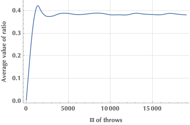
Here is a simple simulation in Mathematica for a rod of length \(L=1\). Notice how the average ratio converges on \(-1 + \ln{4} \simeq 0.386\).
L = 1;
f[x_] := x/(L - x)
sim[n_] :=
 Mean[
  f /@ RandomReal[{0, L/2},   n]
  ]
ListPlot[
 Table[{n, sim[n]}, {n, 1, 20000, 1000}], Joined -> True,
 InterpolationOrder -> 2, PlotRange -> All,
 Frame -> {True, True, False, False},
 FrameLabel -> {"# of throws", "Value of ratio"},
 GridLines -> Automatic, PlotRange -> All]
Stuff to think about
- Why is the result independent of the length \(L\)? Is there any intuitive answer to this?
- Why was it enough to integrate from \(x=0\) to \(x=L/2\) and not do something like:
Is there any symmetry in the problem that allows us to shortcut it? (Always look for symmetries!)
- What whould happen if the probability of the rod breaking at some point wasn’t the same along the rod? Say because the rod was weaker as we moved to its left end. How would this affect the symmetry of the initial problem?