Applications of autoencoders
machine learning mathematics neural networks statisticsContents
Introduction
Hello, world! It’s been nine months since my last post! I was so engaged working at Chronicles Health that I couldn’t find time to reserve for blogging. However, the previous week was my last one there. Now I’ll wear my medical hat again and work as a radiation oncology consultant, hopefully enjoying a more predictable work schedule. I will probably write a blog post about my venture working on a startup. But for now, all I wanted was to make a soft comeback by writing a short post on the applications of autoencoders, one of my favorite machine learning topics.
In the future, I expect to find time to expand on these topics via separate posts, with in-depth analysis and coding examples.
Applications of autoencoders
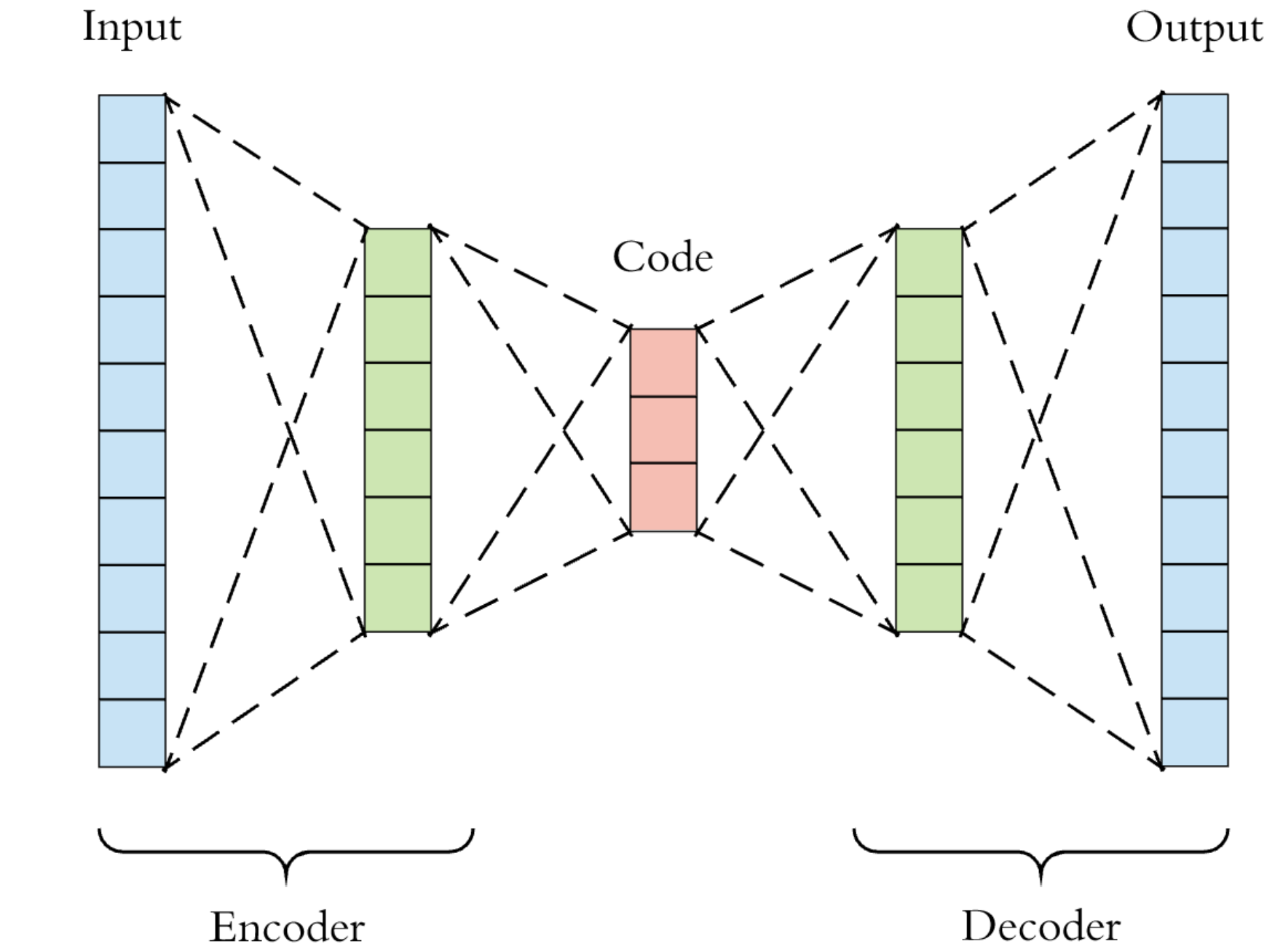
Dimensionality reduction
We have already used autoencoders as a dimensionality reduction technique before, and judging from Google Analytics, this post has been quite a success! So, the idea here is to compress the input by learning some efficient low-dimensional data representation encoded onto the latent layer. To the extent that we accomplish that, we can then replace the original input \(x\) with the new \(x_\text{latent}\), just like we can replace \(x\) with the first couple of principal components when doing PCA.
As it turns out, though, there are quite a few more applications that we will present here briefly.
Feature extraction
To the uninitiated, feature extraction is the process of transforming some data so that the new variables are more informative and less redundant than the original ones. Also, the new derived values (features), hopefully, can differentiate different classes of things in a classification task or predict some target value in a regression task. This application is tightly related to dimensionality reduction. Here’s how we do it. We take raw (unlabelled) data and train an autoencoder with it to force the model learn efficient data representations (the so-called latent space). Once we have trained the autoencoder network, we then ignore the decoder part of the model. Instead, we use only the encoder to convert new raw input data into the latent space representation. This new representation can then be used for supervised learning tasks. So, instead of training a supervised model to learn how to map \(x\) to \(y\), we ask it to map \(x_\text{latent}\) to \(y\).
Object matching
Again, this application is connected to the previous one. Say we’d like to build a search engine for images or songs. We could save all the items in a database and then go through each one, comparing it with our target. But that would be very time-consuming if we did the comparison pixel-by-pixel (or beat-by-beat). Instead, we could run the entire thing in the latent space. Concretely, we would first pass all the known images (or songs) from a trained autoencoder and save their latent space representation (which, by definition, is low dimensional and cheap!) in a database. The position of the input on the latent space is akin to a “signature”. Assuming we would use a 2D latent space, every song in the database would be characterized just by two numbers! Then, given an image (or song) to search for, we would convert it into a latent space representation (again, two numbers), and then we would search the database for it. The comparison could be made via, for instance, the Euclidean distance between the target and the \(i\)-th element in the database. The rationale is that operating on low-dimensional latent space is much more economical, computation-wise, than high-dimensional original space. What if this method doesn’t work? Well, we could try increasing the latent space dimensionality from 2D to 3D and try again until we find the minimum number of dimensions in the latent space that are enough to separate the images (or songs) in our database.
To be a bit more concrete, this is the hypothetical database of known songs along with their latent encoding:
| Song name | Coordinate of latent dim 1 | Coordinate of latent dim 2 |
|---|---|---|
| Enter Sandman | 0.65 | 0.12 |
| Fear of the Dark | 0.44 | 0.99 |
| … | … | … |
| Land of the free | 0.81 | 0.03 |
And suppose we are given an unknown song with \(\text{coord latent dim}_1 = 0.45, \text{coord latent dim}_2 = 0.97\). We would then calculate its distance from the first, 2nd, 3rd song in the database, and we would pick the one with the minimum distance. Neat?
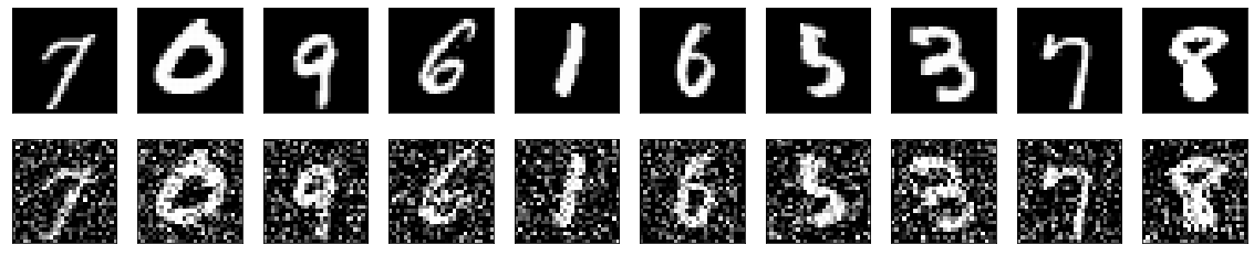
Denoising
Autoencoders can be trained in such a way that they learn how to perform efficient denoising of the source. Contrary to conventional denoising techniques, they do not actively look for noise in the data. Instead, they extract the source from the noisy input by learning a representation of it. The representation is subsequently used to decompress the input into noise-free data. A concrete example is training an autoencoder to remove noise from images. The key to accomplishing this is to take the training images, add some noise to them, and use them as the \(x\). Then use the original images (without the noise) as the \(y\). So, to put it a bit more formally, we are asking the network to learn the mapping \((x+\text{noise}) \to x\). The following figure is taken from Keras’s documentation on autoencoders. The upper row consists of the original untainted images (the \(y\)), and the lower row contains images with some noise added by us (the \(x\)).
Anomaly detection
Since autoencoders are trained to reconstruct their input as well as they can, naturally, if they are given an out of distribution example, the reconstruction will not be as good as if this example was from the training distribution. So, by using some proper threshold for the reconstruction loss, one can build an anomaly detector: any outlier \(x\) will be reconstructed as \(x'\), where \(\left|x' - x\right| \gt \text{thresh}\).
Synthetic data generation
Variational autoencoders can generate new synthetic data, primarily images but also time series. The way to do this is by first training an autoencoder with some data and then randomly sampling the latent dimension of the autoencoder. These random samples are then handed over to the decoder part of the network, leading to new data generation. The following image shows the results of sampling an autoencoder trained on the MNIST dataset. These digits do not exist in the training dataset; they are generated by the network.
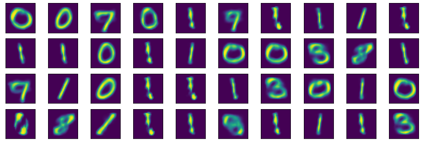
Variational autoencoders differ from vanilla autoencoders because the network learns a (typically) normal distribution for the latent vectors. This acts as some sort of regularization since autoencoders tend to memorize their input.
Data imputation
This is similar to the previous application. The idea here is to take a dataset without any missing entries and randomly delete some of the rows for some of the columns, pretending they are missing. However, we know the ground truth values and train the autoencoder to output those. Once trained, we can present a really missing entry to the network, and assuming that it has been trained robustly, it should perform efficient imputation. Again, to be a bit more concrete, given a dataset with \(x\) values without any missing data, we artificially remove some values and then train an autoencoder to learn the mapping \(x_{\text{missing}} \to x\).
Image colorization
Image colorization is the process of assigning colors to a grayscale image.
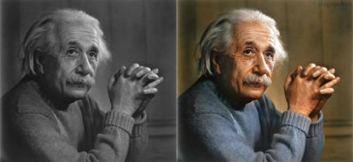
This task can be achieved by taking a dataset with colored images and creating a new dataset with pairs of grayscale and colored images. We then train an autoencoder to learn the mapping \(x_\text{grayscale} \to x_\text{colored}\).