Bayesian optimization for hyperparameter tuning
algorithms Bayes theorem neural networks optimization programming PythonContents
Introduction
Plot: We died and ended up in Dante’s inferno – the optimization version. So, what does it mean to be in an optimization hell?
We are asked to optimize a function we don’t have an analytic expression for. It follows that we don’t have access to the first or second derivatives, hence using gradient descent or Newton’s method is a no-go. Also, we don’t have any convexity guarantees about \(f(x)\). Therefore, methods from the convex optimization field are also not available to us. The only thing we can do is to evaluate \(f(x)\) at some \(x\)’s. However, as if the situation was not bad enough, the function we want to optimize is very costly. So, we can’t just go ahead and massively evaluate \(f(x)\) in, say, 100 billion random points and keep the one \(x\) that optimizes \(f(x)\)’s value.
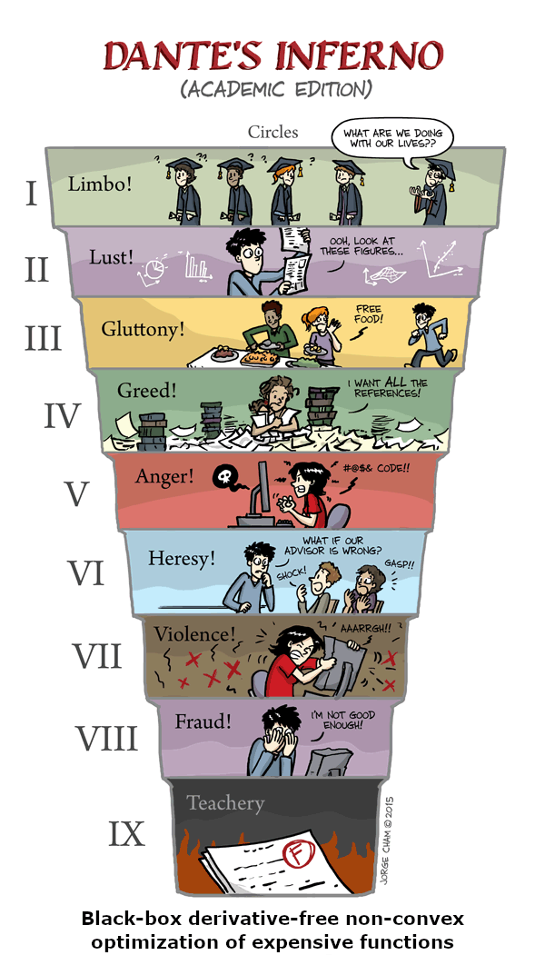
To summarize, we want to optimize an expensive, black-box, derivative-free, possibly non-convex function. And for this kind of problem, Bayesian Optimization (BO) is a universal and robust method.
Mind that the evaluation of the objective function is not necessarily computational! Let me give you a couple of examples, where \(f(x)\) is not something you can calculate with a computer:
- You are a researcher investigating mixtures of chemotherapeutic drugs for their ability to kill cancer cells. You have narrowed it down to three candidate molecules, and you need to find the best combination of concentrations \(c_1, c_2, c_3\) of the three drugs. Evaluating the objective function \(f(c_1,c_2,c_3)\) in this context entails conducting actual experiments in the lab requiring personnel, consumables, and waiting for hours or days for the cell cultures to grow. Therefore, considering all possible concentration combinations is not a realistic approach. Instead, you need to begin with a few random drug concentrations, test them, and then use the experimental outcomes to predict the most promising drug combination to use next. Makes sense?
- You work as a consultant for an oil company, and you want to maximize a probability density function \(f({\tiny\text{LAT}, \tiny\text{LONG}})\) of finding oil if you drill on \(({\tiny\text{LAT}, \tiny\text{LONG}})\) coordinates. Here, the evaluation of the function at a point requires the conduction of actual drilling. And this costs lots of money; therefore, you need to make good educated guesses, and you need to do so with only a few trials.
In other cases, however, \(f(x)\) is indeed be computational. For instance, we may define it as the k-fold cross-validation error of a machine-learning model whose hyperparameters we want to tune. As a matter of fact, we will do precisely this later on.
The ingredients of Bayesian Optimization
Surrogate model
Since we lack an expression for the objective function, the first step is to use a surrogate model to approximate \(f(x)\). It is typical in this context to use Gaussian Processes (GPs), as we have already discussed in a previous blog post. It’s vital that you grasp the concept of GPs, and then BO will require almost no mental effort to sink. There are other choices for surrogate models, but let’s stick to GPs for now. Once we have built a proxy model for \(f(x)\), we want to decide which point \(x\) to sample next. This is the responsibility of the acquisition function (AF), which kind of “peeks” at the GP and generates the best guess \(x\). So, in BO, there are two main components: the surrogate model, which most often is a Gaussian Process modeling \(f(x)\), and the acquisition function that yields the next \(x\) to evaluate. Having said that, a BO algorithm would look like this in pseudocode:
- Evaluate \(f(x)\) at \(n\) initial points
- While \(n \le N\) repeat:
- Update the surrogate model (e.g., the GP posterior) using all available data \(\mathcal{D}_{1:n}\)
- Compute the acquisition function,\(u(x\mid\mathcal{D}_{1:n})\), using the current surrogate model
- Let \(x_{n+1}\) be the maximizer of the acquisition function, i.e. \(x_{n+1} = \text{argmax}_x u(x\mid\mathcal{D}_{1:n})\)
- Evaluate \(y_{n+1} = f(x_{n+1})\)
- Augment the data \(\mathcal{D}_{1:n+1} = \{\mathcal{D}_{1:n}, (x_{n+1}, y_{n+1})\}\) and increment \(n\)
- Return either the \(x\) evaluated with the largest \(f(x)\), or the point with the largest posterior mean.
Acquisition function
As we have already noted, the purpose of the acquisition function is to guide the next best point to sample \(f(x)\). Acquisition functions are constructed so that a high value corresponds to potentially high values of the objective function. Either because the prediction is high or because the uncertainty is high. Which is why they favor regions that already correspond to optimal values or areas that haven’t been explored yet. This is known as the so-called exploration-exploitation trade-off.
If you have played strategy games, like Age of Empires or Command & Conquer, you are already familiar with the concept. Initially, we are placed at some part of the map, and only the immediate area is visible to us. We may choose to sit there and mine any resources we already have access to or send a scouter to explore the invisible part of the map. By exploring the map, we risk meeting the enemy and getting killed, but also, we may find some high-value resources.

To find the next point to evaluate, we optimize the acquisition function. This an optimization problem itself, but luckily it does not require the evaluation of the objective function. In some cases, we may even derive an exact equation for the AF and find a solution with, say, gradient-based optimization. There are three often cited acquisition functions: expected improvement (EI), maximum probability of improvement (MPI), and upper confidence bound (UCB). Although often mentioned last, I think it’s best to talk about UCB because it contains explicit exploitation and exploration terms:
\[a_{\text{UCB}}(x;\lambda) = \mu(x) + \lambda \sigma(x)\]With UCB, the exploitation vs. exploration trade-off is explicit and easy to tune via the parameter \(\lambda\). Concretely, we construct a weighted sum of the expected performance captured by \(\mu(x)\) of the Gaussian Process, and of the uncertainty \(\sigma(x)\), captured by the standard deviation of the GP. Assuming a small \(\lambda\), BO will favor solutions that are expected to be high-performing, i.e., have high \(\mu(x)\). Conversely, high values of \(\lambda\) will make BO favor the exploration of currently uncharted areas in the search space.
Here is an example of a Gaussian Process along with a corresponding acquisition function. This is a 1-dimensional optimization problem, but the idea is the same for more variables. The black dots are our measurements, i.e. the \(x\)’s where we have already sampled \(f(x)\). The black dotted line is the objective function, and the black solid line is our surrogate model of it, i.e., our posterior Gaussian Process. The blue shaded area represents the uncertainty of our surrogate model, \(\sigma(x)\), corresponding to regions in the domain of the objective function that we don’t have any observations. The green line is the acquisition function, which informs us what point \(x\) to sample next. Notice that it takes high values in regions where our GP’s \(\mu(x)\) is high and \(\sigma(x)\) is high.
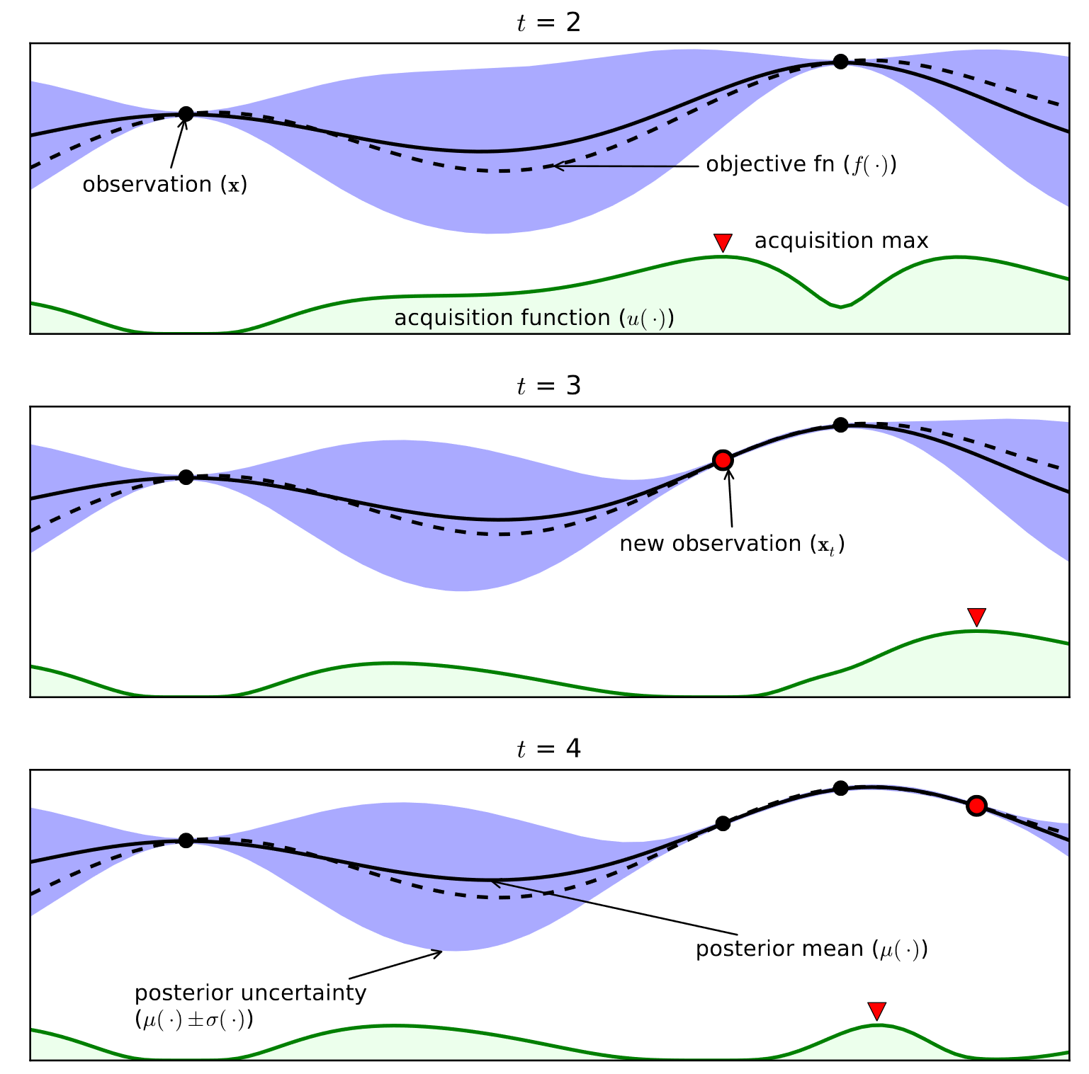
Image taken from here.
This was a lightweight introduction to how a Bayesian Optimization algorithm works under the hood. Next, we will use a third-party library to tune an SVM’s hyperparameters and compare the results with some ground-truth data acquired via brute force. In the future, we will talk more about BO, perhaps by implementing our own algorithm with GPs, acquisition functions, and all.
Hyperparameter tuning of an SVM
Let’s import some of the stuff we will be using:
from sklearn.datasets import make_classification
from sklearn.model_selection import cross_val_score
from sklearn.svm import SVC

import matplotlib.pyplot as plt
import matplotlib.tri as tri
import numpy as np
from hyperopt import fmin, tpe, Trials, hp, STATUS_OK
Create a dataset
Then, we construct an artificial training dataset with many classes, where some of the features are informative, and some are not:
# Create a random n-class classification problem.

# n_features is the total number of features
# n_informative is the number of informative features
# n_redundant features are generated as random linear combinations of the informative features

X_train, y_train = make_classification(n_samples=2500, n_features=20, n_informative=7, n_redundant=3)
Objective function definition
In this example, we will be using the hyperopt package to perform the hyperparameter tuning. First, we define our objective/cost/loss function. This is the \(f(\mathbf{x})\) that we want talked about in the introduction, and \(\mathbf{x} = [C, \gamma]\) is the parameter space. Therefore, we want to find the best combination of \(C, \gamma\) values that minimizes \(f(\mathbf{x})\). The machine learning model that we will be using is a Support Vector Machine (SVM), and the loss will be derived from the average 3-fold cross-validation score.
def objective(args):
    '''Define the loss function / objective of our model.

    We will be using an SVM parameterized by the regularization parameter C
    and the parameter gamma.

    The C parameter trades off correct classification of training examples
    against maximization of the decision function's margin. For larger values
    of C, a smaller margin will be accepted.

    The gamma parameter defines how far the influence of a single training
    example reaches, with larger values meaning 'close'.
    '''
    C, gamma = args
    model = SVC(C=10 ** C, gamma=10 ** gamma, random_state=12345)
    loss = 1 - cross_val_score(estimator=model, X=X_train, y=y_train, scoring='roc_auc', cv=3).mean()
    return {'params': {'C': C, 'gamma': gamma}, 'loss': loss, 'status': STATUS_OK }
Optimization
Now, we will use the fmin() function from the hyperopt package. In this step, we need to specify the search space for our parameters, the database in which we will be storing the evaluation points of the search, and finally, the search algorithm to use. The careful reader might notice that we are doing 1000 evaluations, although we said that evaluation \(f(x)\) is expensive. That’s correct; the only reason we do so is because we want to exaggerate the effect of exploitation vs. exploration, as you shall see in the plots.
trials = Trials()
best = fmin(objective,
    space=[hp.uniform('C', -4., 1.), hp.uniform('gamma', -4., 1.)],
    algo=tpe.suggest,
    max_evals=1000,
    trials=trials)
Let’s print the results:
print(best)
100%|██████████| 1000/1000 [13:01<00:00,  1.28trial/s, best loss: 0.046323449153816476]
{'C': 0.7280999882033379, 'gamma': -1.6752085795502363}
Let us now extract the value of our objective function for every \(C, \gamma\) pair:
# Extract the loss for every combination of C, gamma
results = trials.results
ar = np.zeros(shape=(1000,3))
for i, r in enumerate(results):
    C = r['params']['C']
    gamma = r['params']['gamma']
    loss = r['loss']
    ar[i] = C, gamma, loss
And then use it to plot the loss surface:
C, gamma, loss = ar[:, 0], ar[:, 1], ar[:, 2]

fig, ax = plt.subplots(nrows=1)
ax.tricontour(C, gamma, loss, levels=14, linewidths=0.5, colors='k')
cntr = ax.tricontourf(C, gamma, loss, levels=14, cmap="RdBu_r")

fig.colorbar(cntr, ax=ax)
ax.plot(C, gamma, 'ko', ms=1)
ax.set(xlim=(-4, 1), ylim=(-4, 1))
plt.title('Loss as a function of $10^C$, $10^\gamma$')
plt.xlabel('C')
plt.ylabel('gamma')

plt.show()
Brute-force evaluation of objective function
Since the parameter space is just 2-dimensional, the dataset relatively small, and the SVM training fast, we can brute-force compute the value of the objective function for all possible values of \(C\) and \(\gamma\). These will be our ground-truth data against which we will compare the results from the BO run.
def sample_loss(args):
    C, gamma = args
    model = SVC(C=10 ** C, gamma=10 ** gamma, random_state=12345)
    loss = 1 - cross_val_score(estimator=model, X=X_train, y=y_train, scoring='roc_auc', cv=3).mean()
    return loss

lambdas = np.linspace(1, -4, 25)
gammas = np.linspace(1, -4, 20)
param_grid = np.array([[C, gamma] for gamma in gammas for C in lambdas])

real_loss = [sample_loss(params) for params in param_grid]
And here is the respective contour plot:
C, G = np.meshgrid(lambdas, gammas)
plt.figure()
cp = plt.contourf(C, G, np.array(real_loss).reshape(C.shape), cmap="RdBu_r")
plt.colorbar(cp)
plt.title('Loss as a function of $10^C$, $10^\gamma$')
plt.xlabel('$C$')
plt.ylabel('$\gamma$')
plt.show()
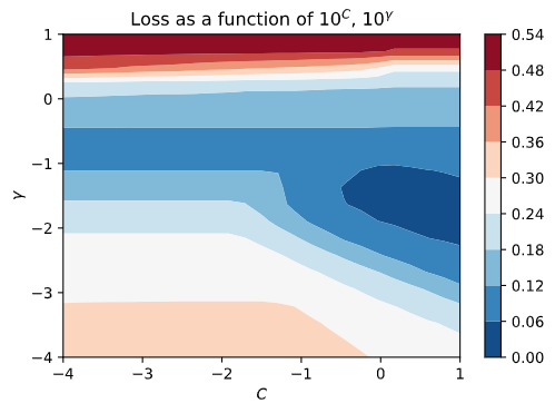
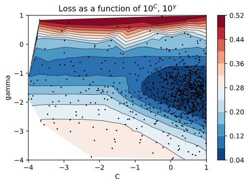
Let’s place the two plots side-by-side and talk about the results. In the left image, we see the ground-truth values of the loss function that we acquired by computing the value \(\ell(C, \gamma)\) for every possible pair of \((C, \gamma)\) via a grid-search. You see the blue shaded region corresponding to low values for the loss function (good!) and the red stripe at the top corresponding to high values for the loss function (bad!). In the right image, we see the black points corresponding to our tried values. Do you notice how there is a high density of points near the blue shaded area where \(\ell(C,\gamma)\) is minimized? That’s exploitation! The BO algorithm picked up some good solutions into that area and sampled aggressively around that region. On the contrary, it tried some values near the top red stripe region, and since those trials yielded bad results, it didn’t bother sampling any further there.
| Ground-truth values | Bayesian Optimization |
|---|---|
|
|
References
- https://thuijskens.github.io/2016/12/29/bayesian-optimisation/