Acquisition functions in Bayesian Optimization

Contents

• Introduction
• A schematic Bayesian Optimization algorithm
• Acquisition Functions
  • Upper Confidence Bound (UCB)
  • Probability of Improvement (PI)
  • Expected Improvement (EI)

Introduction

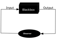
In a previous blog post, we talked about Bayesian Optimization (BO) as a generic method for optimizing a black-box function, \(f(x)\), that is a function whose formula we don’t know. The only thing we can do in this setup is to ask \(f\) evaluate at some \(x\) and observe the output.

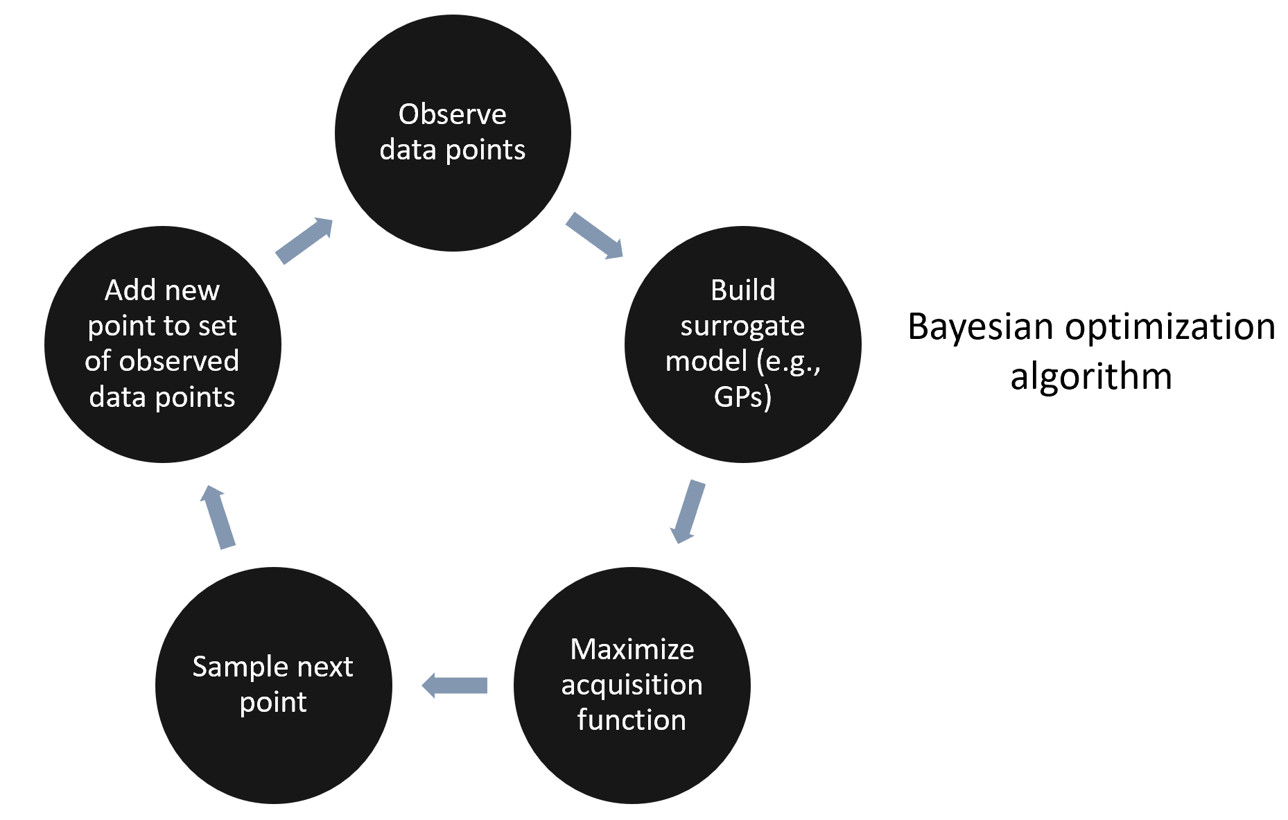
A schematic Bayesian Optimization algorithm

The essential ingredients of a BO algorithm are the surrogate model (SM) and the acquisition function (AF). The surrogate model is often a Gaussian Process that can fit the observed data points and quantify the uncertainty of unobserved areas. So, SM is our effort to approximate the unknown black-box function \(f(x)\).

Next, the acquisition function “looks” at the SM and determines what areas in the domain of \(f(x)\) are worth exploiting and what areas are worth exploring. Accordingly, in areas where \(f(x)\) is optimal or areas that we haven’t yet looked at, AF assumes a high value. On the contrary, in areas where \(f(x)\) is suboptimal or areas that we have already sampled from, AF’s value is small. By finding the \(x\) that maximizes the acquisition function, we identify the next best guess for \(f\) to try. That’s right: instead of maximizing directly \(f(x)\), whose analytic form we don’t even know, we instead maximize another function, AF, that is much easier to do and much less expensive. So, the steps that a BO algorithm follows are the following.

In the following video, we demonstrate the exploitation (trying slightly different things that have already been proven to be good solutions) vs. exploration (trying totally different things from areas that have not yet been probed) tradeoff. Although here \(f(x)\) is known, in the general case, it is not.

Acquisition Functions

Upper Confidence Bound (UCB)

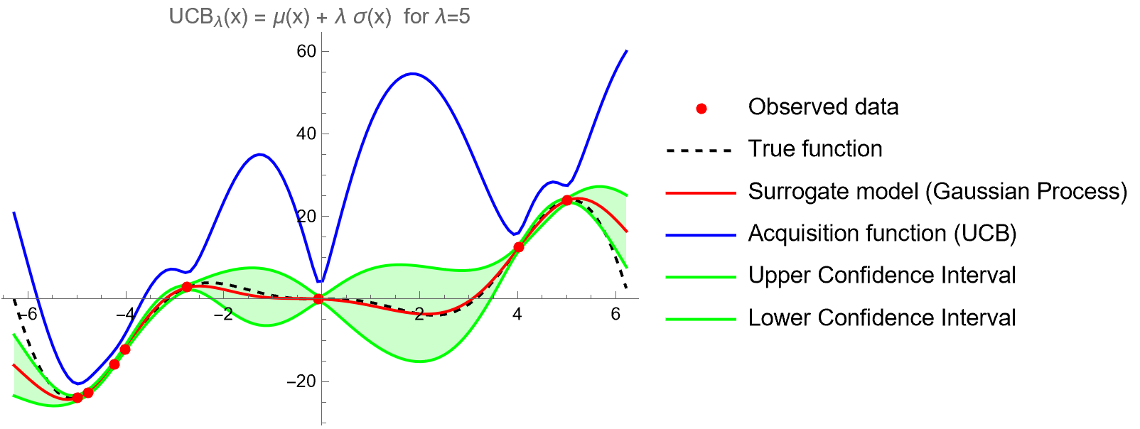
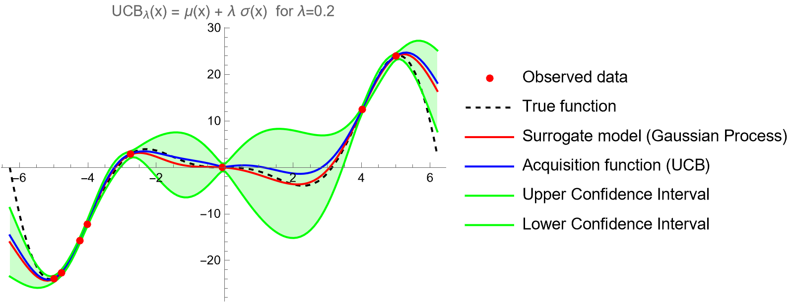
Probably as simple as an acquisition function can get, upper confidence bound contains explicit exploitation (\(\mu(x)\)) and exploration (\(\sigma(x)\)) terms:

\[a(x;\lambda) = \mu(x) + \lambda \sigma (x)\]

With UCB, the exploitation vs. exploration tradeoff is straightforward and easy to tune via the parameter \(\lambda\). Concretely, UCB is a weighted sum of the expected performance captured by \(\mu(x)\) of the Gaussian Process, and of the uncertainty \(\sigma(x)\), captured by the standard deviation of the GP. When \(\lambda\) is small, BO will favor solutions that are expected to be high-performing, i.e., have high \(\mu(x)\). On the contrary, when \(\lambda\) is large, BO rewards the exploration of currently uncharted areas in the search space.

Here is an example with a large value for \(\lambda\). UCB favors areas where we don’t have any samples from.

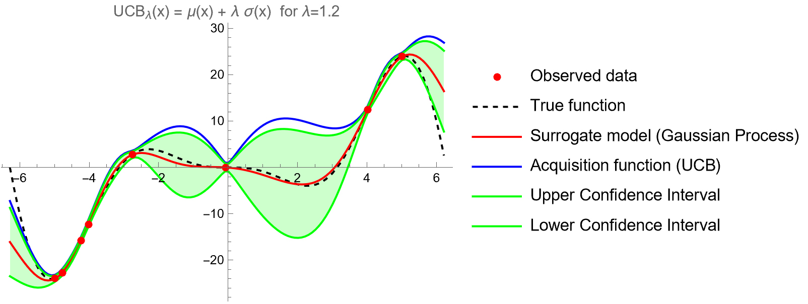
This is an example with a value for \(\lambda\) around 1 (I made \(\lambda=1.2\) so that AF and upper confidence interval curves don’t coincide). UCB balances between known good values and unexplored areas.

Finally, here is an example with a small value for \(\lambda\). UCB is very conservative in this case and will cause aggressive sampling around the current best solution.

Probability of Improvement (PI)

Suppose that we’d like to maximize \(f(x)\), and the best solution we have so far is \(x^\star\). Then, we can define “improvement”, \(I(x)\), as:

\[I(x) = \max(f(x) - f(x^\star), 0)\]

Therefore, if the new \(x\) we are looking at has an associated value \(f(x)\) that is less than \(f(x^\star)\), then \(f(x) - f(x^\star)\) is negative. So we aren’t improving at all, and the above formula returns 0, since the maximum number between any negative number and 0 is 0. On the contrary, if the new value \(f(x)\) is larger than our current best estimate, then \(f(x) - f(x^\star)\) is positive. In this case \(I(x)\) returns the difference which is how much we will improve over our current best solution if we evaluate \(f\) at the new point \(x\).

In probability of improvement acquisition function, for each candidate \(x\) we assign the probability of \(I(x)>0\), i.e., \(f(x)\) being larger than our current best \(f(x^\star)\). Let us recall that in a Gaussian Process, at each point there’s a Gaussian distribution attached. Therefore, at point \(x\) the value of the function \(f(x)\) is sampled from a normal distribution with mean \(\mu(x)\) and variance \(\sigma^2(x)\):

\[f(x) \sim \mathcal{N}(\mu(x), \sigma^2(x))\]

Now, let us use a reparameterization trick. If \(z \sim \mathcal{N}(0, 1)\), then \(f(x) = \mu(x) + \sigma(x) z\) is a normal distribution with mean \(\mu(x)\) and variance \(\sigma^2(x)\). Therefore, we can rewrite the improvement function, \(I(x)\), as:

\[I(x) = \text{max}(f(x) - f(x^\star), 0) = \text{max}(\mu(x) + \sigma(x) z - f(x^\star), 0) \,\, z \sim \mathcal{N}(0,1)\]

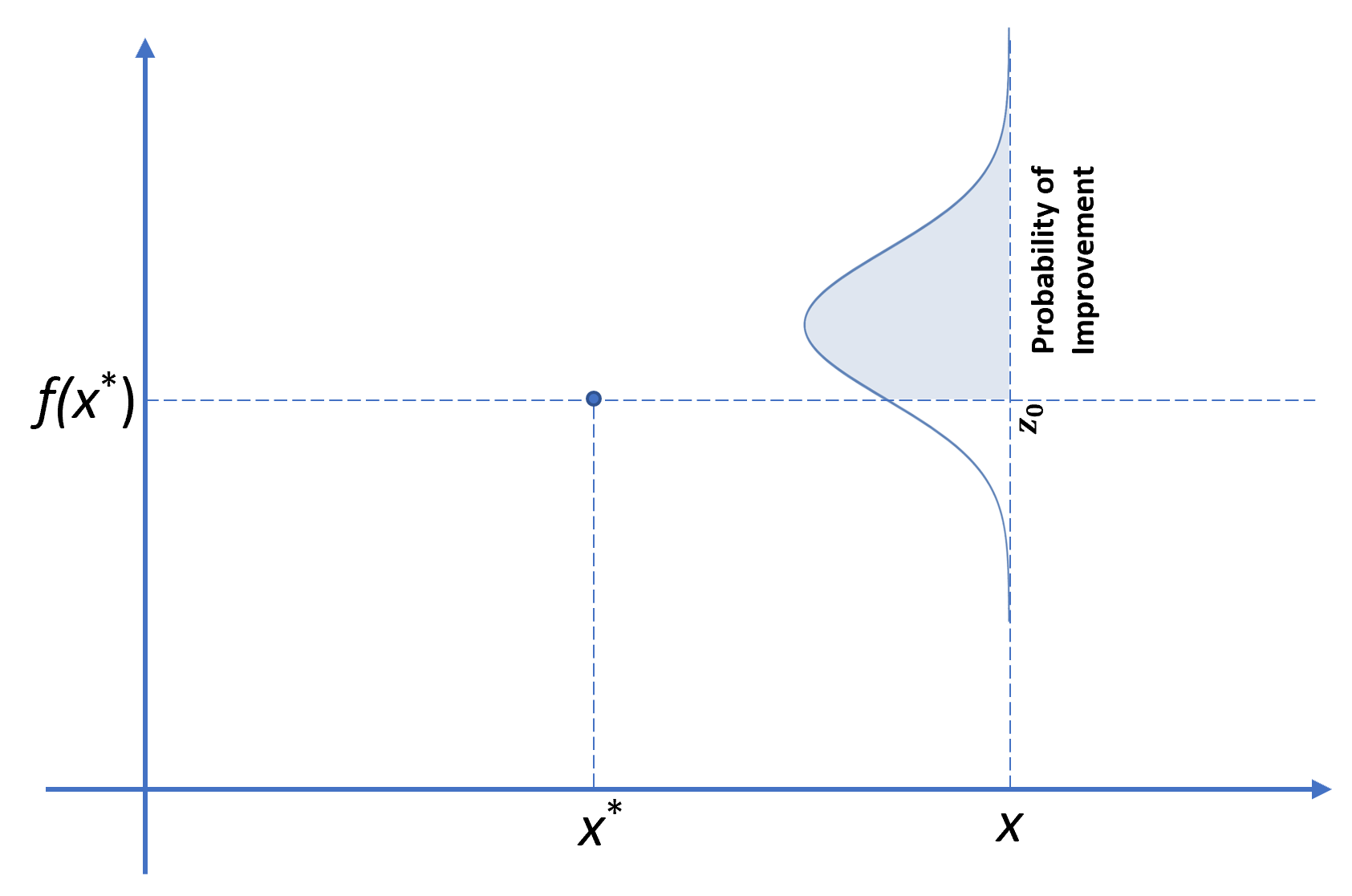
Let us take a pause here and make sure that we really understand what’s going on. Here \(x\) is some point that we want to check whether it worths evaluating \(f\) at. So, we assign a value \(I(x)\) to it. However, \(I(x)\)’s value is sampled from a normal distribution \(\mathcal{N}(\mu(x), \sigma^2(x))\). So, here’s how we calculate:

\[\text{PI}(x) = \text{Pr}(I(x) > 0) \Leftrightarrow \text{Pr}(f(x) > f(x^\star))\]

If you look at the image above, it’s clear that the probability of improvement is the shaded area under the Gaussian curve for \(z>z_0\). Therefore:

\[\text{PI}(x) = 1 - \Phi(z_0) = \Phi(-z_0) = \Phi\left(\frac{\mu(x)-f(x^\star)}{\sigma(x)}\right)\]

Where \(\Phi(z) \equiv \text{CDF}(z)\) and \(z_0 = \frac{f(x^\star) - \mu(x)}{\sigma(x)}\).

Expected Improvement (EI)

PI considers only the probability of improving our current best estimate, but it does not factor in the magnitude of the improvement. This is where the expected improvement acquisition function is different. Instead of looking at the improvement \(I(x)\), which is a random variable, we will instead calculate the “Expected Improvement”, which is the expected value of \(I(x)\):

\[\text{EI}(x)\equiv\mathbb{E}\left[I(x)\right] = \int_{-\infty}^{\infty} I(x)\varphi(z) \mathop{\mathrm{d}z}\]

Where \(\varphi(z)\) is the probability density function of the normal distribution \(\mathcal{N}(0,1)\), i.e., \(\varphi(z) = \frac{1}{\sqrt{2\pi}}\exp\left(-z^2/2\right)\). In case you aren’t familiar with the expected value of a random variable, it’s kind of a weighted average of “value” times “probability of getting that value”.

Ok, so:

\[\text{EI}(x) = \int_{-\infty}^{\infty} I(x)\varphi(z) \mathop{\mathrm{d}z}=\int_{-\infty}^{\infty}\underbrace{\max(f(x) - f(x^\star), 0)}_{I(x)}\varphi(z)\mathop{\mathrm{d}z}\]

How do we calculate this integral? We need to get rid of the \(max\) operator. In order to do that, we are going to break up the integral into two components, one where \(f(x) - f(x^\star)\) is positive and one where it is negative. The point where the switch happens is given by:

\[f(x) = f(x^\star) \Rightarrow \mu + \sigma z = f(x^\star) \Rightarrow z = \frac{f(x^\star) - \mu}{\sigma}\]

Let’s call this point \(z_0 = \frac{f(x^\star) - \mu}{\sigma}\), and break up the integral as:

\[\text{EI}(x) = \underbrace{\int_{-\infty}^{z_0} I(x)\varphi(z) \mathop{\mathrm{d}z}}_{\text{Zero since }I(x)=0} + \int_{z_0}^{\infty} I(x)\varphi(z) \mathop{\mathrm{d}z}\]

Ok, so we are good to go now:

\[\begin{aligned} \text{EI}(x) &=\int_{z_0}^{\infty} \max(f(x)-f(x^\star),0) \varphi(z)\mathop{\mathrm{d}z} = \int_{z_0}^{\infty} \left(\mu+\sigma z - f(x^\star)\right)\varphi(z) \mathop{\mathrm{d}z}\\ &= \int_{z_0}^{\infty} \left(\mu - f(x^\star) \right)\varphi(z)\mathop{\mathrm{d}z} + \int_{z_0}^{\infty} \sigma z \frac{1}{\sqrt{2\pi}}e^{-z^2/2}\mathop{\mathrm{d}z} \\\\ &=\left(\mu- f(x^\star)\right) \underbrace{\int_{z_0}^{\infty}\varphi(z)\mathop{\mathrm{d}z}}_{1-\Phi(z_0)\equiv 1-\text{CDF}(z_0)} + \frac{\sigma}{\sqrt{2\pi}}\int_{z_0}^{\infty} z e^{-z^2/2}\mathop{\mathrm{d}z}\\ &=\left(\mu- f(x^\star)\right) (1-\Phi(z_0)) - \frac{\sigma}{\sqrt{2\pi}}\int_{z_0}^{\infty} \left(e^{-z^2/2}\right)' \mathop{\mathrm{d}z}\\ &=\left(\mu- f(x^\star)\right) (1-\Phi(z_0)) - \frac{\sigma}{\sqrt{2\pi}} \left[e^{-z^2/2}\right]_{z_0}^{\infty}\\ &=\left(\mu- f(x^\star)\right) \underbrace{(1-\Phi(z_0))}_{\Phi(-z_0)} + \sigma \varphi(z_0) \\ &=\left(\mu- f(x^\star)\right) \Phi\left(\frac{\mu-f(x^\star)}{\sigma}\right) + \sigma \varphi\left(\frac{\mu - f(x^\star)}{\sigma}\right) \end{aligned}\]

At the last point, we used the fact that the PDF of normal distribution is symmetric, therefore \(\phi(z_0) = \phi(-z_0)\). Alright, so this equation might seem intimidating, but it’s really not. So, when does \(\text{EI}(x)\) take high values? When \(\mu > f(x^\star)\). I.e., then mean value of the Gaussian Process is high at \(x\). Expected improvement is also increased when there’s lots of uncertainty, therefore when \(\sigma > 1\). By the way, the formula above works for \(\sigma(x)>0\), otherwise, if \(\sigma(x) = 0\) (as it happens at the observed data points), it holds that \(\text{EI}(x)=0\).

There’s one last before we conclude. By injecting a (hyper)parameter \(\xi\) into the formula for \(\text{EI}(x)\), we can fine tune how much exploitation vs. how much exploration the BO algorithm will do. So, the full formula is:

\[\text{EI}(x;\xi) = \left(\mu- f(x^\star) - \xi\right) \Phi\left(\frac{\mu-f(x^\star)-\xi}{\sigma}\right) + \sigma \varphi\left(\frac{\mu - f(x^\star)-\xi}{\sigma}\right)\]

For \(\xi=0\), we just end up with the previous formula. However, for large values of \(\xi\), you can think of it as if we pretend to have a larger current best value than we actually do! Therefore, this steers the BO algorithm towards more exploration.