Introduction

What is EM about?

Maximum likelihood estimation (MLE)

The expectation-maximization (EM) algorithm is an iterative method to find the local maximum likelihood of parameters in statistical models. So what is the maximum likelihood? It’s the maximum value of the likelihood function! And what is a likelihood function? It’s a function of the model’s parameters treating the observed data as fixed points, i.e., we write \(\mathcal{L}(\theta\mid x)\) meaning that we vary the parameters \(\theta\) while taking the \(x\)’s as given. If \(\mathcal{L}(\theta_1\mid x) > \mathcal{L}(\theta_2 \mid x)\) then the sample we observed is more likely to have occurred if \(\theta = \theta_1\) rather than if \(\theta = \theta_2\). So, given the data that we have observed, the likelihood function points to a model’s most plausible parameterization that might have generated the observed data.

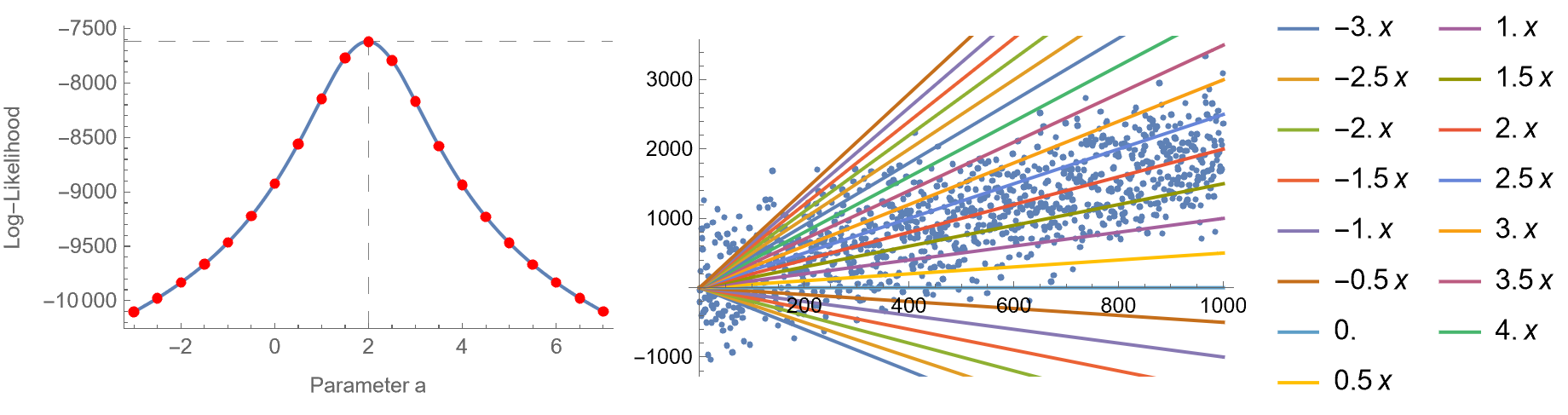
Here is an elementary example. Suppose that we have some data and want to fit a model of the form \(y = a x\). In this case, \(\theta\) is essentially the coefficient \(a\), but usually, there will be many unknown parameters. In the left image, there’s the likelihood function for several values of the parameter \(a\) (actually, it’s the logarithm of the likelihood function, but we will talk about this later). In the right image, we plot \(y = a x, \, a = -3, \ldots 7\) with a step size of 0.5, superimposed with the observed data. As you can see, \(a = 2\) maximizes the log-likelihood and fits the data better than any other line. So, fitting data to models can be done via maximum likelihood estimation.

Log likelihood of linear regression model

By the way, in a previous blog post we have proven that by maximizing the likelihood in the linear regression case, this is equivalent to minimizing the mean squared error.

… in the presence of hidden variables

The EM algorithm is particularly useful when there are missing data in the data set or when the model depends on hidden or so-called latent variables. These are variables that affect our observed data but in ways that we can’t know directly. So what’s so special about latent parameters? Typically, if we know all the parameters, we can take the derivatives of the likelihood function with respect to them, solve the system of equations and find the values that maximize the likelihood. Like:

\[\left\{\frac{\partial \mathcal{L}}{\partial \theta_1}=0, \frac{\partial \mathcal{L}}{\partial \theta_2}=0, \ldots \right\}\]

This is precisely what we did when we wanted to fit some data to a normal distribution. However, in statistical models with latent variables, this typically results in a set of equations where the solutions to the parameters mandate the values of the latent variables and vice versa. By substituting one set of equations into the other, an unsolvable equation is produced. That’s why we need the expectation-maximization algorithm. Concretely, EM can be used in any of the following scenarios:

Estimating parameters of (usually Gaussian) mixture models
Estimating parameters of Hidden Markov Models
Unsupervised learning of clusters
Filling missing data in samples

What are the basic steps of EM?

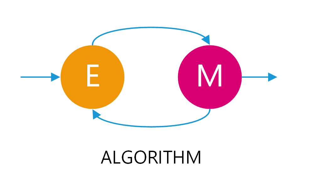
Expectation-Maximization algorithm schematic

EM takes its name from the alternation between two algorithmic steps. The first step is the expectation step, where we form a function for the expectation of the log-likelihood, using the current best estimates of the model’s parameters. Whereas, in the maximization step, we calculate the new parameters’ values by maximizing the expected log-likelihood. These new estimates of the parameters are then used to determine the distribution of the latent variables in the next expectation step. Don’t worry if it doesn’t make sense now; we will show an example in a minute, and we will also delve into it in subsequent blog posts.

A 1-dimensional example

Setting up the problem

Let us consider some observed 1-dimensional data points, \(x_i\). We assume they are generated by two normal distributions \(N(\mu_1, \sigma_1^2)\) and \(N(\mu_2, \sigma_2^2)\), with probabilities \(\pi\) and \(1-\pi\), respectively. In this setup, we have 5 unknown parameters: the mixing probability \(\pi\), the mean and standard deviation of the first distribution, and the mean and standard deviation of the second distribution. Let us gather all these under a vector called \(\theta = [\pi, \mu_1, \sigma_1, \mu_2, \sigma_2]\).

Histogram of mixed gaussian distribution

Writing down the likelihood function

Suppose that we observed a datapoint with value \(x_i\). What is the probability of \(x_i\) occuring? Assuming \(\varphi_1(x)\) is the probability density function of the 1st distribution, and \(\varphi_2(x)\) of the second, the probability of observing \(x_i\) is:

\[p(x_i) = \pi \varphi_1(x_i) + (1-\pi)\varphi_2(x_i)\]

To be more pedantic we would write:

\[p(x_i\mid \theta) = \pi \varphi_1(x_i \mid \mu_1,\sigma_1^2) + (1-\pi)\varphi_2(x_i \mid \mu_2,\sigma_2^2)\]

Which means that the PDF’s are paremeterized by \(\mu_1,\sigma_1^2\) and \(\mu_2, \sigma_2^2\), respectively. Ok, but this is just for a single observation \(x_i\). What if we have a bunch of \(x_i\)’s, say for \(i=1,\ldots,N\)? To find the joint probability of \(N\) independent events (which by the way is the likelihood function!) we just multiply the individual probabilities:

\[\mathcal{L}(\theta \mid x) = \prod_{i=1}^N p(x_i \mid \theta)\]

But since it’s easier to work with sums rather than products, we take the logarirthm of the likelihood, \(\ell(\theta\mid x)\):

\[\begin{align*}\ell(\theta \mid x) &= \log \prod_{i=1}^N p(x_i \mid \theta) =\sum_{i=1}^N \log p(x_i \mid \theta)\\&=\sum_{i=1}^N \log \left[\pi \varphi_1(x_i\mid \mu_1,\sigma_1^2) + (1-\pi)\varphi_2(x_i|\mu_2,\sigma_2^2)\right]\end{align*}\]

So, our objective is to maximize likelihood \(\mathcal{L}(\theta\mid x)\), which is equivalent to maximizing the log-likelihood \(\ell(\theta\mid x)\), with respect to the model’s parameters \(\theta = [\pi, \mu_1, \sigma_1, \mu_2, \sigma_2]\), given the data points \(\{x_i\}\).

Brute forcing one parameter at a time

In the following examples, we will generate some synthetic observed data from a mixture distribution with known parameters \(\mu_1, \sigma_1, \mu_2, \sigma_2\) and mixing probability \(\pi\). We will then calculate \(\ell(\theta\mid x)\) for various parameter values while keeping the rest of the parameters fixed. Every time we will do that, we will see how \(\ell(\theta\mid x)\) is maximized when a model’s parameter becomes equal to its ground-truth value.

Let’s create a mixture distribution of two Gaussian distributions with known parameters \(\mu_1, \sigma_1, \mu_2, \sigma_2\) and known mixing probability \(\pi=0.3\). Normally, we won’t know the values of these parameters, and as a matter of fact, finding them will be the very objective of the EM algorithm. But for now, let’s pretend we don’t know them.

ClearAll["Global`*"];
{m1, s1} = {1, 2};
{m2, s2} = {9, 3};

npts = 5000;
dist[m_, s_] := NormalDistribution[m, s];
mixdist[p_] :=
 MixtureDistribution[{p, 1 - p}, {dist[m1, s1], dist[m2, s2]}]
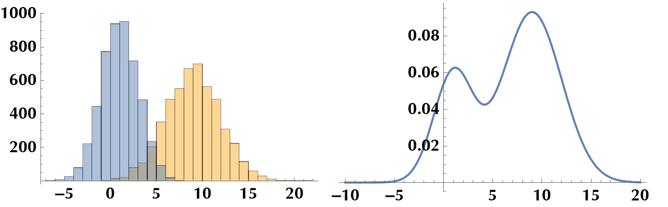
data = RandomVariate[mixdist[0.3], npts];
Histogram[data]

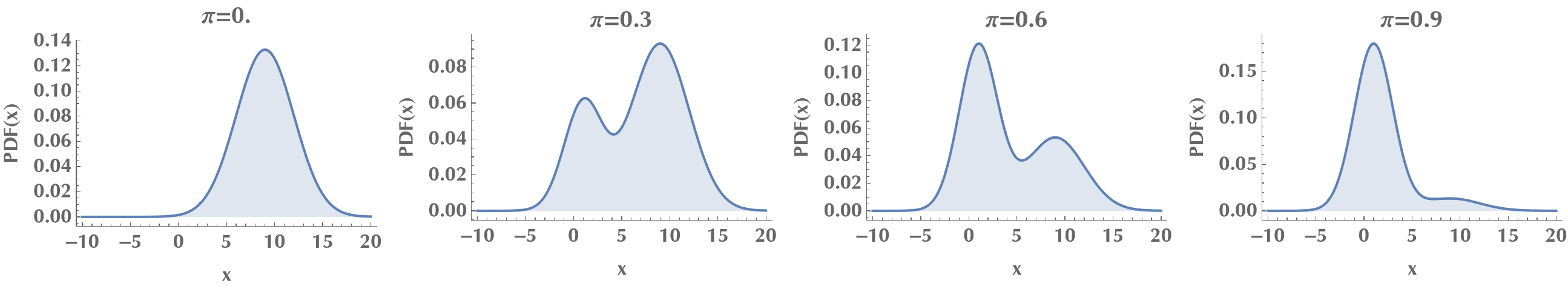
Histogram of mixture distribution

Let’s plot the probability density functions of the mixture distribution for various mixing probabilities \(\pi\). We notice how for \(\pi\to 0\) the mixture distribution approaches the 1st distribution, and for \(\pi\to 1\), the 2nd distribution. For in-between values, it’s a mixture! ;)

Style[Grid[{
   Table[
    Plot[PDF[mixdist[p], x], {x, -10, 20}, 
     PlotLabel -> "p=" <> ToString@p,
     FrameLabel -> {"x", "PDF(x)"}, 
     Frame -> {True, True, False, False},
     AxesOrigin -> {-10, 0}, Filling -> Axis],
    {p, 0, 1, 0.3}]
   }],
 ImageSizeMultipliers -> 0.7]

PDF of mixture distribution for varying mixing probability

Let us now define the log-likelihood function:

logLikelihood[data_, p_, m1_, s1_, m2_, s2_] :=
 Module[{},
  Sum[
   Log[
    p PDF[dist[m1, s1], x] + (1 - p) PDF[dist[m2, s2], x] /. 
     x -> data[[i]]
    ],
   {i, 1, Length@data}]
  ]

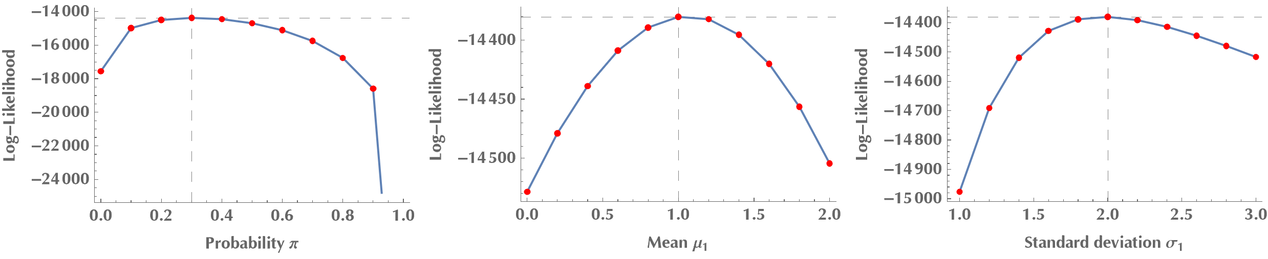
Ok, we are ready to go. We will first vary the mixing probability \(\pi\), keeping the rest of the model’s parameters fixed. In some sense, we are brute-forcing \(\pi\), to find \(\pi\):

llvalues = 
  Table[{p, logLikelihood[data, p, m1, s1, m2, s2]}, {p, 0, 1, 0.1}];
{pmax, llmax} = 
 llvalues[[Ordering[llvalues[[All, 2]], -1][[1]]]]
(* {0.3, -14437.1} *)

plot1 =
 Show[
  ListPlot[llvalues, Joined -> True, 
   FrameLabel -> {"Probability p", "Log-Likelihood"}, 
   Frame -> {True, True, False, False}, 
   GridLines -> {{pmax}, {llmax}}, GridLinesStyle -> Dashed],
  ListPlot[llvalues, PlotStyle -> {Red, AbsolutePointSize[5]}]
  ]

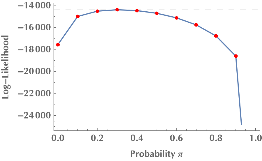
Log likelihood for varying mixing probability

Do you see how \(\ell(\theta\mid x)\) is maximized at \(\pi = 0.3\)? By the same token, we can try other model parameters, but we will always come to the same conclusion: the log-likelihood, therefore the likelihood, is maximized when our guesses become equal to the ground-truth values for the model’s parameters.

Log likelihood for varying mixing probability, mean and standard deviation

Reformulating the problem as a latent variable problem

Previously, we varied one parameter at a time, keeping the rest at their ground-truth values. We will now get serious and seek to estimate the values of all parameters simultaneously. If we attempt to directly maximize \(\ell(\theta|x)\), it will be tough due to the sum of terms inside the logarithm. For those of you who doubt it, just calculate the partial derivatives of \(\ell(\theta|x)\) with respect to \(\pi, \mu_1, \sigma_1, \mu_2, \sigma_2\) and contemplate solving the system where all these derivatives are required to become zero. Good luck with that! :P

There’s another way to go, though. We will reformulate our problem as a problem of maximum likelihood estimation with latent variables. For this, we will introduce a set of latent variables called \(\Delta_i \in \{0,1\}\). If \(\Delta_i = 0\) then \(x_i\) was sampled from the 1st distribution, and if \(\Delta_i = 1\), then it came from the 2nd distribution. In this case, the log-likelihood \(\ell(\theta\mid x,\Delta)\) is given by:

\[\begin{align*} \ell(\theta\mid x,\Delta) = &\sum_{i=1}^N \left[ (1-\Delta_i) \log \varphi_1(x_i) + \Delta_i \log\varphi_2(x_i)\right] +\\ &\sum_{i=1}^N \left[ (1-\Delta_i)\log\pi + \Delta_i\log(1-\pi)\right] \end{align*}\]

When we write \(\varphi_1(x_i)\) in reality we mean \(\varphi_1(x_i\mid \mu_1, \sigma_1^2)\), and similarly for \(\varphi_2(x_i)\) we mean \(\varphi_2(x_i\mid \mu_2, \sigma_2^2)\). The reason we omited it, is for keeping the log-likelihood expression easily readable. Feel free to check that the above formula is equal to the previous expression of \(\ell(\theta\mid x)\), by first letting \(\Delta_i = 0\) and then \(\Delta_i = 1\).

But, we don’t actually know the values \(\Delta_i\). After all, these are the latent variables that we introduced into the problem! If you feel that we ain’t making any progress, hold on. Here’s where the EM algorithm kicks in. Even though we don’t know the exact values \(\Delta_i\), we will use their expected values given our current best estimates for the model’s parameters! This is the expectation step of the EM algorithm. So, instead of \(\Delta_i\), we will use \(\gamma_i\) defined as:

\[\gamma_i(\theta) = \mathbb{E}(\Delta_i\mid \theta,x) = \text{Pr}(\Delta_i = 1\mid \theta,x)\]

Once we have \(\gamma_i\) calculated, we know which distribution \(x_i\) belongs to. Therefore, we can update the model’s parameters using the weighted maximum-likelihood fits. For Gaussian distributions, this is just the mean and standard deviation of the \(x_i\). This is the maximization step! Actually, \(\gamma_i\) doesn’t take discrete values like the \(\Delta_i\). Instead, it lies in the interval \([0,1]\) and, therefore, the EM algorithm does a soft membership assignment. I.e., for every \(x_i\), it assigns a probability that it comes from the 1st or the 2nd distribution. That’s why, when we calculate the Gaussians’ parameters, we use a \(\gamma_i\)-weighted average.

EM algorithm

So, here’s the EM algorithm for our particular problem:

Initialize unknown parameters (e.g., \(\hat{\pi} = 0.5, \hat{\mu_1} = \text{random }x_i, \sigma_i = \sum_{i=1}^N(x_i-\bar{x})^2/N, \ldots\)
Expectation step:

\[\hat{\gamma_i} = \frac{(1-\pi) \varphi_2(x_i)}{\pi \varphi_1(x_i) + (1-\pi)\varphi_2(x_i)}\]

Maximization step:

\[\begin{align*} \hat{\mu_1} &= \frac{\sum_{i=1}^N (1-\hat{\gamma_i})x_i}{\sum_{i=1}^N (1-\hat{\gamma_i})}\hspace{3cm}\hat{\mu_2} = \frac{\sum_{i=1}^N \hat{\gamma_i} x_i}{\sum_{i=1}^N \hat{\gamma_i}}\\ \hat{\sigma_1} = &\sqrt{\frac{\sum_{i=1}^N (1-\hat{\gamma_i})(x_i-\hat{\mu_1})^2}{\sum_{i=1}^N (1-\hat{\gamma_i})}}\hspace{1cm} \hat{\sigma_2} = \sqrt{\frac{\sum_{i=1}^N \hat{\gamma_i}(x_i-\hat{\mu_2})^2}{\sum_{i=1}^N \hat{\gamma_i}}}\\ \hat{\pi} &= \sum_{i=1}^N(1-\hat{\gamma_i})/N \end{align*}\]

Repeat until convergence or maximum number of iterations reached.

Here is a sample code that implements the EM algorithm for our particular problem. The code doesn’t look pretty without Mathematica’s syntax color highlighting and the Notebook’s format, but anyway.

em[data_, p_, m1_, s1_, m2_, s2_] :=
 Module[{newp, newm1, news1, newm2, news2, g, npts},
  npts = Length@data;
  g = Table[((1 - p) PDF[dist[m2, s2], data[[i]]]) / (p PDF[dist[m1, s1], data[[i]]] + (1 - p) PDF[dist[m2, s2], data[[i]]]), {i, 1, npts}];
  newm1 = Sum[(1 - g[[i]])*data[[i]], {i, 1, npts}] / Sum[1 - g[[i]], {i, 1, npts}];
  newm2 = Sum[g[[i]]*data[[i]], {i, 1, npts}] / Sum[g[[i]], {i, 1, npts}];
  news1 = Sqrt[Sum[(1 - g[[i]])*(data[[i]] - m1)^2, {i, 1, npts}] / Sum[1 - g[[i]], {i, 1, npts}]];
  news2 = Sqrt[Sum[g[[i]]*(data[[i]] - m2)^2, {i, 1, npts}] / Sum[g[[i]], {i, 1, npts}]];
  newp = Sum[(1 - g[[i]])/npts, {i, 1, npts}];
  {newp, newm1, news1, newm2, news2, g}
  ]

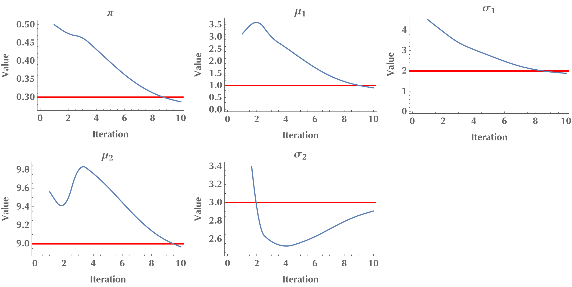
doEM[data_] :=
 Module[{p, m1, s1, m2, s2, g},
  {p, m1, s1, m2, s2} = {0.5, RandomChoice[data], StandardDeviation[data], RandomChoice[data], StandardDeviation[data]};
  Print[{p, m1, s1, m2, s2}];
  For [i = 1, i < 40, i++,
   {p, m1, s1, m2, s2, g} = em[data, p, m1, s1, m2, s2];
   If[Mod[i, 4] == 0, Print[{p, m1, s1, m2, s2}]]
   ];
  {p, m1, s1, m2, s2, g}
  ]

This is a short test run, where we confirm that the algorithm converges to the ground-truth values (the red lines are the ground-truth values). As we mentioned in the introduction, EM is a local algorithm, meaning it can get stuck at a local maximum. Therefore, sometimes we may need to repeat the algorithm a few times to ensure a near-global optimal solution.

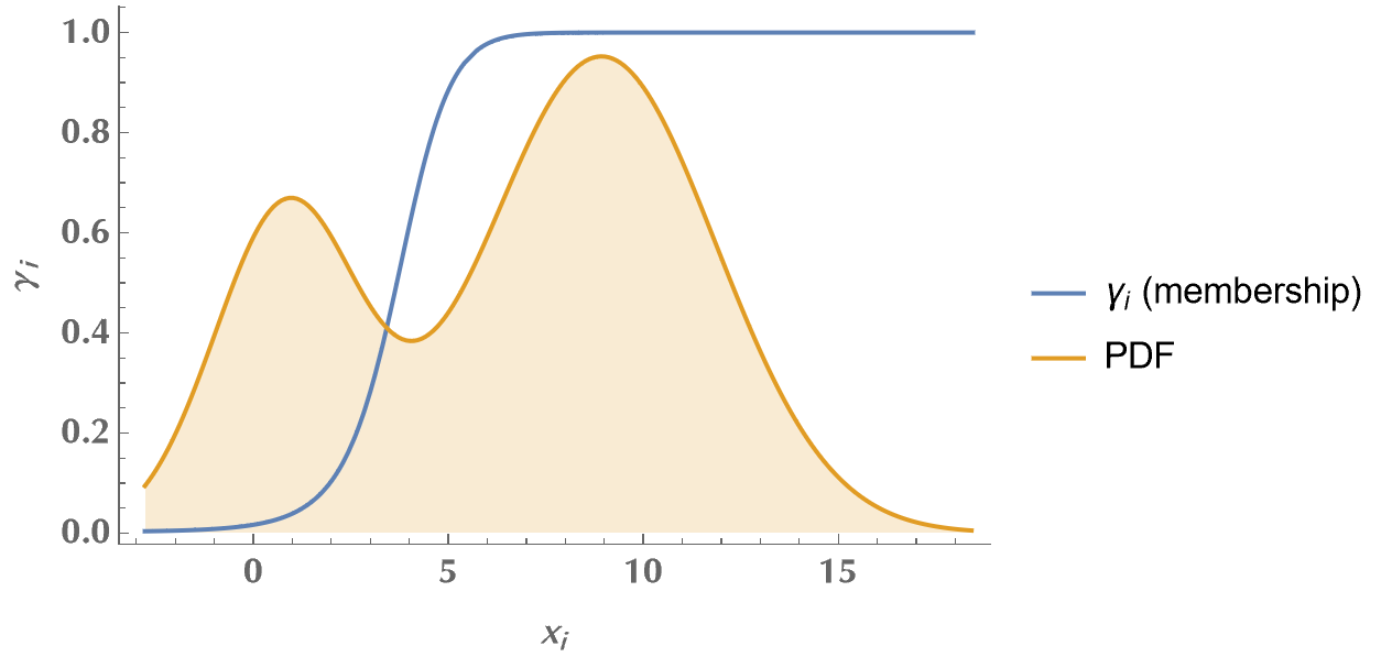
Expectation Maximization algorithm for Gaussian mixture models

In the following plot, we see how the \(\gamma_i\)’s vary as the observed data transition from the 1st to the 2nd distribution. E.g., when we look at observed data around x=1 (or less), the \(\gamma_i\)’s are equal to zero. This means that the EM algorithm doesn’t cast any doubt on the source of these values. They were sampled from the 1st distribution. When we look at observed data around x=9 (or more), EM is confident that these values originate from the second distribution (\(\gamma_i=1\)). However, when we are in between, \(\gamma_i\)’s assume intermediate values around 0.5, conveying the uncertainty regarding which distribution each \(x_i\) belongs to. So, by applying the EM algorithm, we discovered the membership of each observed value (with some uncertainty), and we estimated the model’s unknown parameters! Neat?