Custom training loops with Pytorch
machine learning mathematics neural networks pytorch statisticsContents
Introduction
In a previous post, we saw a couple of examples on how to construct a linear regression model, define a custom loss function, have Tensorflow automatically compute the gradients of the loss function with respect to the trainable parameters, and then update the model’s parameters. We will do the same in this post, but we will use PyTorch this time. It’s been a while since I wanted to switch from Tensorflow to Pytorch, and what better way than start from the basics?
Fit quadratic regression model to data by minimizing MSE
Generate training data
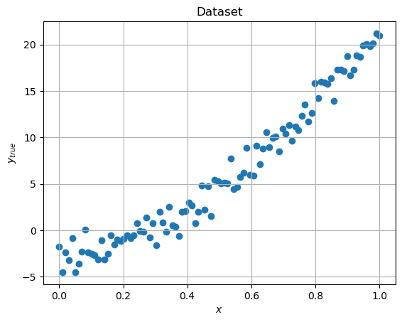
First, we will generate some data coming from a quadratic model, i.e., \(y = a x^2 + b x + c\), and we will add some noise to make the setup look a bit more realistic, as in the real world.
import torch
import matplotlib.pyplot as plt

def generate_dataset(npts=100):
    x = torch.linspace(0, 1, npts)
    y = 20*x**2 + 5*x - 3
    y += torch.randn(npts)  # Add some noise
    return x, y

x, y_true = generate_dataset()

plt.scatter(x, y_true)
plt.xlabel('$x$')
plt.ylabel('$y_{true}$')
plt.grid()
plt.title('Dataset')
Define a model with trainable parameters
In this step, we are defining a model, specifically the \(y = f(x) = a x^2 + b x + c\). Given the model’s parameters, \(a, b, c\), and an input \(x\), \(x\) being a tensor, we will calculate the output tensor \(y_\text{pred}\):
def f(x, params):
    """Calculate the model's output given a set of parameters and input x"""
    a, b, c = params
    return a * (x**2) + b * x + c
Define a custom loss function
Here we define a custom loss function that calculates the mean squared error between the model’s predictions and the actual target values in the dataset.
def mse(y_pred, y_true):
    """Returns the mean squared error between y_pred and y_true tensors"""
    return ((y_pred - y_true)**2).mean()
We then assign some initial random values to the parameters \(a, b, c\), and also tell PyTorch that we want it to compute the gradients for this tensor (the parameters tensor).
params = torch.randn(3).requires_grad_()
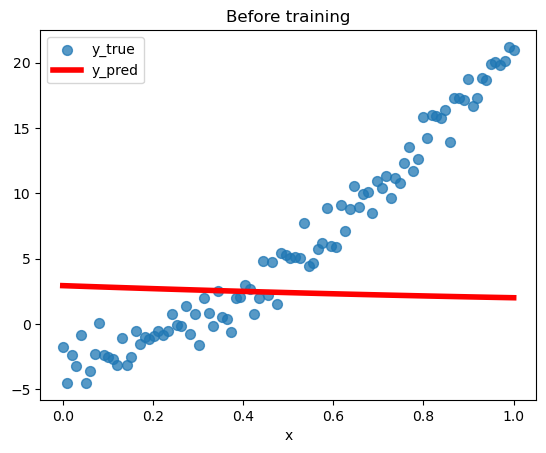
y_pred = f(x, params)Here is a helper function that draws the predictions and actual targets in the same plot. Before training the model, we expect a considerable discordance between these two.
def plot_pred_vs_true(title):
    plt.scatter(x, y_true, label='y_true', marker='o', s=50, alpha=0.75)
    plt.plot(x, y_pred.detach().numpy(), label='y_pred', c='r', linewidth=4)
    plt.legend()
    plt.title(title)
    plt.xlabel('x')

plot_pred_vs_true('Before training')
Define a custom training loop
This is the heart of our setup. Given the old values for the model’s parameters, we construct a function that calculates its predictions, how much they deviate from the actual targets, and modifies the parameters via gradient descent.
def apply_step():
    lr = 1e-3                                   # Set learning rate to 0.001
    y_pred = f(x, params)                       # Calculate the y given x and a set of parameters' values
    loss = mse(y_pred=y_pred, y_true=y_true)    # Calculate the loss between y_pred and y_true
    loss.backward()                             # Calculate the gradient of loss tensor w.r.t. graph leaves
    params.data -= lr * params.grad.data        # Update parameters' values using gradient descent
    params.grad = None                          # Zero grad since backward() accumulates by default gradient in leaves
    return y_pred, loss.item()                  # Return the y_pred, along with the loss as a standard Python number
Run the custom training loop
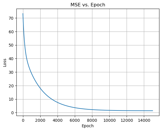
We repeatedly apply the previous step until the training process converges to a particular combination of \(a, b, c\).
epochs = 15000
history = []
for i in range(epochs):
    y_pred, loss = apply_step()
    history.append(loss)

plt.plot(history)
plt.xlabel('Epoch')
plt.ylabel('Loss')
plt.title('MSE vs. Epoch')
plt.grid()
Final results
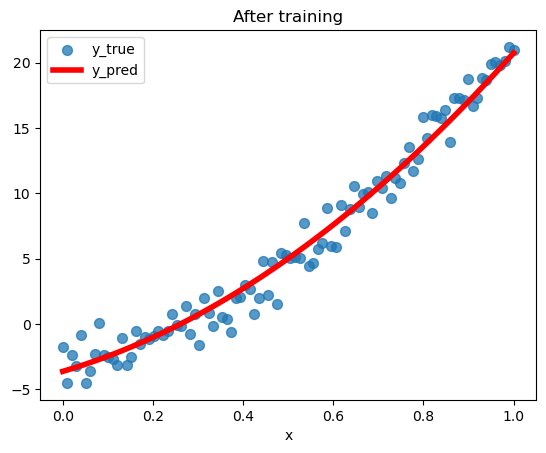
Finally, we superimpose the dataset with the best quadratic regression model PyTorch converged to:
plot_pred_vs_true('After training')