2 Introduction

2.1 Prostate Cancer

Prostate cancer (PCa) is the most common cancer among men, second only to skin cancer. This year, an estimated 191.930 men in the United States will be diagnosed with prostate cancer, accounting for 10.6% of all new cancer cases.¹ Radiation therapy (RT), along with surgery and hormonal treatment, is one of the central pillars in managing PCa. During the last years, radiotherapy technology has seen dramatic progression that allowed dose escalation while keeping normal tissue toxicity from bladder and rectum low.^2,3 Nowadays, Intensity Modulated Radiation Therapy (IMRT) and its evolution, Volumetric Modulated Arc Therapy (VMAT), represent the state-of-the-art treatment techniques.⁴

During VMAT radiotherapy, the linear accelerator rotates around the patient and irradiates from different angles with beamlets of varying aperture shape and intensity (Fig. 2.1). The fields’ shape is modulated by a multileaf collimator (MLC) system consisting of a set of pairs of “leaves”, which can move in and out of the beam’s field. This beam modulation results in a dose gradient that conforms tightly to the target volume, and it drops fast inside the surrounding normal tissues. Had it not been for the modern imaging techniques, such as cone-beam computed tomography, that localize the prostate and guide the precise delivery of radiation, this highly conformal treatment would not have been possible.^5,6

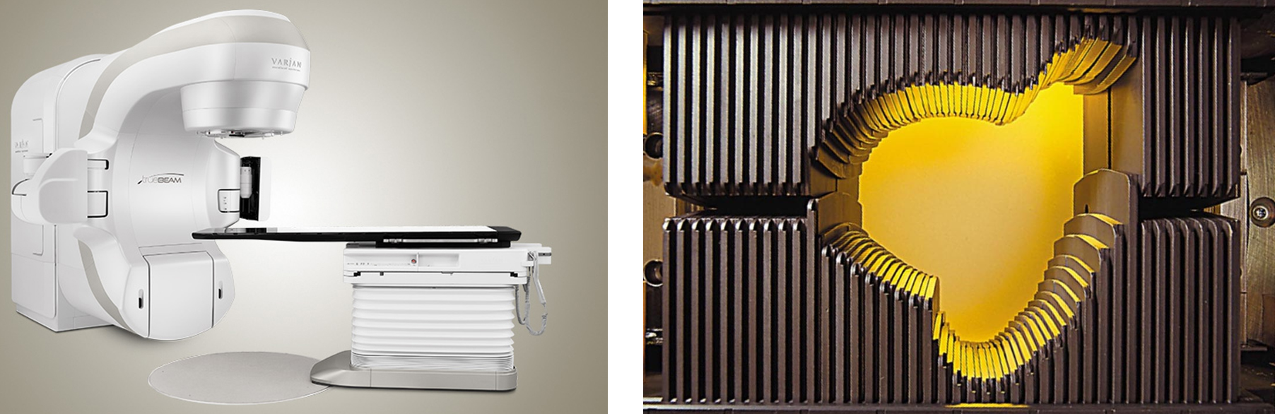
Figure 2.1: Left: A modern linear accelerator able to deliver volumetric modulated arc therapy. Right: A Multi Leaf Collimator (MLC) system. The leaves can move in and out of the beam’s field, shaping the delivered dose.

2.2 Volumetric Modulated Arc Therapy

VMAT, initially introduced under the name IMAT (Intensity Modulated Arc Therapy), was first proposed in 1995,⁷ although another type of IMRT using rotational fan beams was submitted two years earlier by Mackie et al. under the name tomotherapy.⁸ In VMAT, the radiation is delivered over a continuous arc, similar to tomotherapy, but uses rotational cone beams shaped by an MLC system. The idea was to convert the intensity patterns into leaf segments delivered by a sequence of one or more arcs. In principle, one arc would suffice since it may incorporate hundreds of aperture shapes. However, the linear accelerator’s mechanical constraints necessitate multiple arcs to provide additional degrees of freedom to the system. Nowadays, linear accelerators can vary both the dose rate and the gantry speed at each beam angle, besides the aperture shape. These additional modulation degrees allow the creation of sophisticated dose distributions by redistributing the normal tissue dose to less critical regions. Also, partial and non-coplanar arcs can be combined depending on the clinical scenario.

2.3 Inverse treatment planning

IMRT and VMAT treatment planning are inverse compared to conventional 3D conformal radiotherapy workflow. The planning treatment volumes are delineated, along with organs at risks (OARs), prescription and normal tissue constraints are set, and then the optimization algorithm seeks to find the optimal beam delivery. In its simplest form,⁹ the cost function that is optimized is the least square differences between the calculated dose \(d_c(\mathbf{r})\) and the prescribed dose \(d_p(\mathbf{r})\) of structure \(i\), over the 3D dose voxel matrix, weighted by some importance factor \(\lambda_i\):

\[ J \equiv J(\mathbf{w}) = \sum_{i=1}^N \lambda_i \left( d_c(\mathbf{r}) - d_p(\mathbf{r})\right)_i^2 \] There is an abundance of optimization algorithms to minimize the cost function \(J\), such as gradient descent and simulated annealing. In gradient descent, the weights are updated in the direction of the negative gradient of the \(J(\mathbf{w})\), i.e., \(\mathbf{w}_{n+1} = \mathbf{w}_n - \alpha \nabla_{\mathbf{w}}{J}, \alpha>0\). The \(\alpha\) value is the learning rate. The algorithm is iterative and stops when convergence is achieved, i.e., when the gradient \(\nabla_{\mathbf{w}}J(\mathbf{w})\) is so small that \(\mathbf{w}\) does not change much.

In simulated annealing, a parameter (e.g., leaf position, aperture weight) is picked randomly, and its value is changed by some random amount. The new cost function is calculated, and if it is lower \((\Delta J < 0)\), the change is accepted. If the new cost function is higher \((\Delta J > 0)\), then the change is accepted with a probability \(p = \text{min}\left[1,\exp(-\Delta J / T)\right]\), via the criterion \(p \ge u\in[0,1]\), where \(T\) is the annealing temperature that is initialized to some high value and then slowly lowered during the optimization process, and \(u\) a uniform random number \(u\in[0,1]\). The logic behind simulated annealing is that during the initial phase of the optimization process, we want to explore the search space by allowing some suboptimal changes to take place. However, as simulation time passes by, the temperature \(T\) is lowered, which lowers the probability of accepting such solutions, and the algorithm is driven to convergence. In Fig. 2.2 and 2.3 we show two examples, of gradient descent and simulated annealing, minimizing the simple one-dimensional test function from Gramacy and Lee:¹⁰

\[ f(x) = \frac{\sin(10\pi x)}{2x} + (x-1)^4, \hspace{5mm} x \in [0.5, 2.5] \]

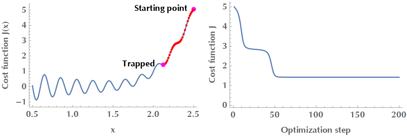
Figure 2.2: Gradient descent is trapped in a local minimum. In order to overcome local minima, there exist versions of gradient descent that use momentum or adaptive learning rate.

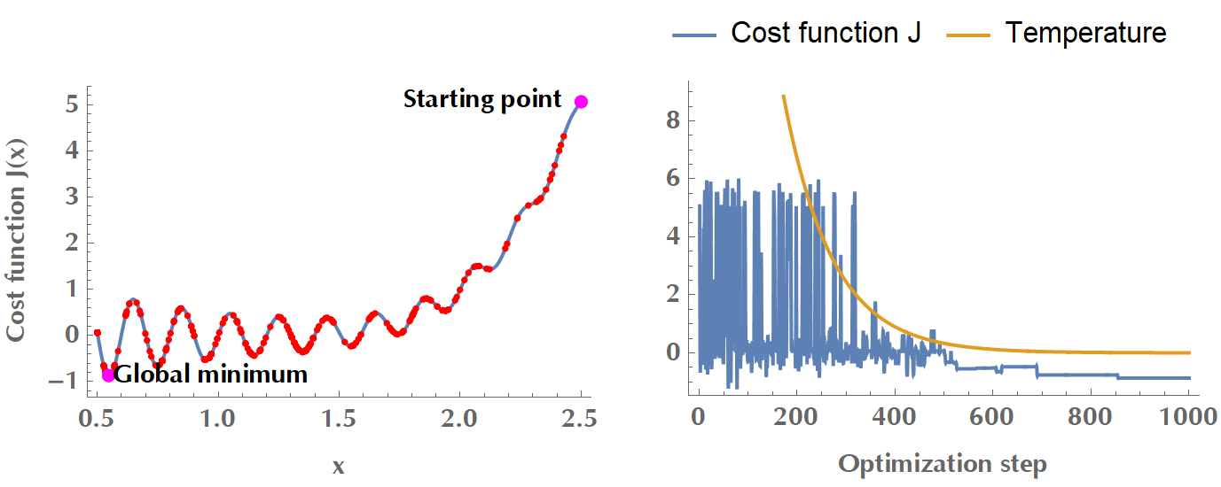
Figure 2.3: Simulated annealing with a cooling schedule \(T(t) = 0.99^t T_0\). During the initial phase of high temperature, the algorithm accepts suboptimal changes to explore the search space. As the temperature drops, the cost function converges to a minimum.

Another versatile method of describing the goodness of treatment of a plan is to use the so-called “costlets”, in which case the overall cost function is given by \(J = F(c_1,c_2,\ldots,c_K)\). The \(c_i, i=1,\ldots,K\) are the costlets and the function \(F\) describes how the various costlets are combined to yield the overall optimization target.¹¹ A natural way to merge the \(c_i\) into a penalty function is to calculate their weighted sum, e.g. \(J=\sum_{i=1}^K \lambda_i c_i\). In this framework, a plan’s complexity could be encoded in a complexity costlet, as per the following simplified example:

\[\begin{align*} J &= 0.2\underbrace{\sum_{i\in SC} \text{max}(d_i - 45, 0)^{10}}_\text{No more than 45 in Spinal Cord} + 0.3\underbrace{\sum_{i\in PTV} \text{max}(d_i - 63, 57 - d_i, 0)^2}_\text{No less than 57 and no more than 63 in PTV} \\ &+ 0.1\underbrace{\sum_{i\in NT} \text{max}(d_i, 0)^2}_\text{Minimize dose to Normal Tissues} + 0.05 \times \text{estimated time of delivery}\\ &+ 0.05 \times \text{tongue & groove effect} + 0.05 \times \text{complexity} + \ldots \end{align*}\]

Once inverse optimization derives an optimal fluence per field, the process is handed over to the “leaf sequencing algorithm” that determines a sequence of leaf motions to deliver that fluence (Fig. 2.4). Naturally, there will be some differences between the “optimal” and “actual” fluence after enforcing the mechanical constraints of the linear accelerator (e.g., maximum leaf speed, limitations in opposing leaf positions). Another strategy is the so-called “Direct Aperture Optimization”, where fluence optimization and leaf positions are optimized directly,¹² therefore what the dosimetrist sees at the optimization stage is what is delivered to the patient.

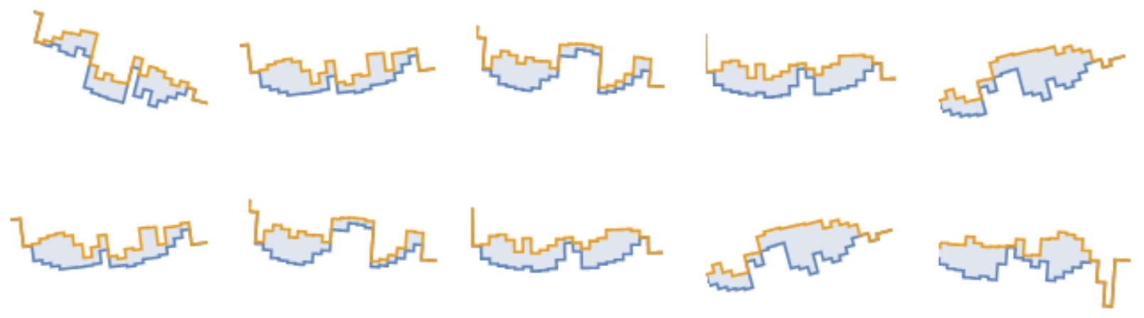
Figure 2.4: Ten reconstructed beamlets (out of total 200) in a VMAT plan. The blue shaded area is the MLC’s aperture. The more irregularly shaped the beamlets, the more complex the plan. Source: Radiation Oncology Department of Papageorgiou General Hospital.

2.4 Plan complexity

VMAT radiation plans are inherently complex to deliver by the linear accelerator. Plan complexity has many reverberations on radiation safety, treatment deliverability, beam-on time, mechanical strain on the linear accelerator, and necessitates laborious quality assurance (QA) and verification procedures.¹³ Concretely, some significant issues arising from excessive complexity include the following:

1. As the number of monitor units (MUs) increases, so does irradiation time and leakage radiation. This “low-dose bath” of normal tissues may double the risk of radiation-induced second cancers.¹⁴

2. Increased overall treatment time might have unfavorable radiobiologic implications in cell-sterilizing ability due to repair of sublethal DNA damage.^15–19

3. The interaction between the delivery of an intricate plan and moving target (such as prostate) is, to a great degree, unknown.

Complexity metrics (CMs) have been suggested as a complementary analytical tool to existing quality controls methods.²⁰ The extra information provided by CMs could facilitate the selection of a robust plan, deliverability-wise, among plans with similar dosimetric characteristics (Fig. 2.5). A complexity metric could also be used as an optimization objective in the treatment planning system to reduce the plan complexity at an early stage.²¹ Integrating complexity minimization at the objective function, rather than at later stages of treatment planning, is advantageous in the following sense. It increases delivery efficiency while maintaining dosimetric quality. On the contrary, other methods, such as beamlet intensity restrictions, smoothing procedures, and direct aperture optimization, may compromise target coverage and OAR sparing in exchange for increased beam smoothness and delivery efficiency.²¹

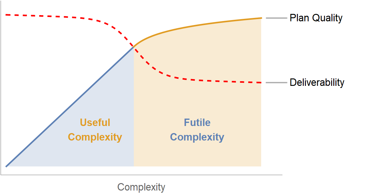
Figure 2.5: Qualitative representation of complexity vs. plan quality and plan deliverability.

However, a high degree of complexity is not a priori a negative feature of a treatment plan. It may be the case that due to the particular target and anatomy of organs at risk, a rather intricate plan needs to be delivered. This may occur around complex targets involving convex and non-convex parts, and a tradeoff between treatment plan quality and required monitor units has been shown in the context of IMRT.²² Therefore, a balance between excessive complexity and dose distribution compromise is the most prudent way forward.