4 Methods

4.1 Dataset curation

Two-hundred and seventeen RT-DICOM² files of VMAT prostate plans were exported from the Varian ARIA (Varian Medical Systems, Palo Alto, CA) oncology information system of the Radiation Oncology Department at Papageorgiou General Hospital. All patients were treated radically during 2017-2020, with a moderately hypofractionated radiotherapy scheme.^34,35 Depending on a patient’s risk, the irradiation field encompassed prostate only (PO), prostate plus seminal vesicles (PSV), or the whole-pelvis (WPRT) (Fig. 4.1). Target volumes and organs at risk were delineated on the reference CT image according to the International Commission of Radiation Unit and Measurement 50 and 62 recommendations.^36,37 PTVs were derived from clinical target volumes with an anisotropic expansion (7mm towards all directions except 5mm towards the rectum).

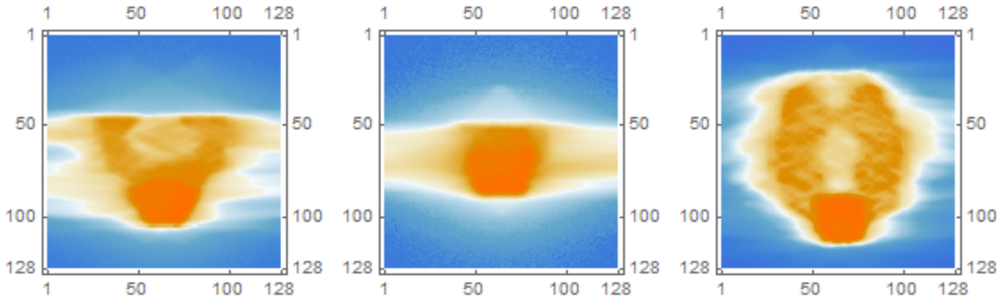
Figure 4.1: Images of 2D dose distributions for prostate plans of various field sizes. From left to right: prostate plus seminal vesicles (PSV), prostate only (PO), and whole pelvis (WPRT). Source: Radiation Oncology Department of Papageorgiou General Hospital.

The plans were created with the Varian Eclipse Treatment Planning System. During the study period, the TPS has undergone a major upgrade from version 11.0.47 to version 15.1.52, which affected the fluence optimization and leaf sequencing algorithms. All VMAT plans were delivered by a 6MV energy linear accelerator (DHX, Varian Medical Systems, Palo Alto, CA) equipped with a 120-leaf MLC (field size 40 \(\times\) 40cm, central 20cm of field - 5mm leaf width, outer 20cm of field - 10mm leaf width), and an on-board imaging kV cone-beam CT system.

The variables of interest were extracted with in-house software under the name rteval (http://test.ogkologia.gr/rteval). The latter can extract a diverse set of radiotherapy parameters from RTDOSE, RTPLAN, and RTSTRUCT DICOM files, such as point dose statistics, clinical dose constraints, arbitrary dose-volume data, contour coordinates, various complexity metrics, and others. The software is written in Python 3 and uses the pydicom library (version 1.3.0). All data were fully anonymized to protect patient anonymity. The research protocol was submitted to the Institutional Review Board of Papageorgiou General Hospital.

4.2 Dataset description

The following data were extracted:

Variables included in the dataset, their type, and a short description of their meaning.

Variable Name	Type	Description
coa	Numerical	Circumference over Area (1/mm)
em	Numerical	Edge Metric (1/mm)
esf	Numerical	Equivalent Square Field (mm)
lt	Numerical	Leaf Travel
ltmcsv	Numerical	Leaf Travel multiplied by MCS-VMAT
mcs	Numerical	Modulation Complexity Score
mcsv	Numerical	Modulation Complexity Score for VMAT plans
mfa	Numerical	Mean Field Area (\(\text{mm}^2\))
pi	Numerical	Plan Irregularity
sas	Numerical	Small Aperture Score at 5 mm
total_mus	Numerical	Total number of monitor units of the plan
arcs	Categorical	The number of beams (1 or 2)
field_size	Categorical	Prostate Only, Prostate plus Seminal Vesicles and Whole Pelvis RT
physician	Categorical	The physician that delineated the tumor volume and organs at risk
dosimetrist	Categorical	The dosimetrist that performed the treatment planning
tps_version	Categorical	The version of Treatment Planning Software
cn	Numerical	Conformation number indicating how tightly dose conforms to target
ptv_72	Numerical	The high-dose (72 Gy) planning treatment volume
bladder_v65	Numerical	The volume of bladder that receives at least 65 Gy
bladder_v70	Numerical	The volume of bladder that receives at least 70 Gy
rectum_v60	Numerical	The volume of rectum that receives at least 60 Gy
rectum_v65	Numerical	The volume of rectum that receives at least 65 Gy
rectum_v70	Numerical	The volume of rectum that receives at least 70 Gy

1. Complexity metrics. The complexity metrics have been described in the literature section of the thesis.
2. Total monitor units. This is the sum of the monitor units of all plan’s beams.
3. Physician. In total, seven physicians delineated tumor volumes and organs at risk. Their usernames haven been replaced by the string \(\text{Phys}_i, i = 1,\ldots,7\) to protect anonymity.
4. Dosimetrist. In total, two dosimetrists optimized the plans. Their usernames have been replaced by the string \(\text{Dos}_i, i = \{1,2\}\) to protect anonymity.
5. TPS version. Plans from two different versions of the Varian Eclipse TPS entered the study, version 11.0.47 and version 15.1.52.
6. Conformation Number (CN). This index measures how tightly the dose distribution conforms around the target.³⁸ It is given by the following equation: \[ \text{CN} = \frac{\text{TV}_{RI}}{\text{TV}} \times \frac{\text{TV}_{RI}}{\text{V}_{RI}} \] where \(\text{TV}\) corresponds to the target volume, \(\text{TV}_{RI}\) to the target Volume covered by some reference isodose (RI), and \(\text{V}_{RI}\) to the volume of the reference isodose. CN consists of two factors, with the first fraction describing the quality of target coverage, whereas the second one the volume of normal tissue receiving a dose equal or greater to a reference dose. A value of 1 represents a reference isodose covering the target volume without irradiation of normal tissues and corresponds to optimal conformation. A value of zero implies a total absence of conformation. We used 95% of the prescribed dose level for the high-dose (72 Gy) PTV as the reference dose to apply the van’t Reit’s formula.³⁸
7. High-dose (72 Gy) PTV. In our department, a moderately hypofractionated scheme is used, where the prostate is receiving 72 Gy in 32 fractions with 2.25 Gy/fraction, seminal vesicles 57.6 Gy with 1.8 Gy/fraction, and pelvic lymph nodes 51.2 Gy with 1.6 Gy/fraction.
8. Dose-volume constraints. These constraints allow only a certain percentage of an organ’s volume (e.g., bladder or rectum) to receive doses above some prespecified threshold level. They have for some time been considered as a de facto standard clinical tool for plan evaluation.³⁹

4.3 Data analysis

After their extraction, the data were tabulated in a Microsoft Excel spreadsheet. The statistical analysis was done in R language version 3.6.3.⁴⁰ Some prototyping and exploratory analyses were performed with Wolfram Mathematica version 12.1, Python version 3.6.9, and scikit-learn version 0.23. The results of the principal component analysis were independently verified with IBM SPSS version 25. This thesis was written in Bookdown,^41,42 an R package built on top of R Markdown, that allows reproducible research. Unless otherwise specified in the text, the level of statistical significance was set at a=0.05.

4.3.1 Summary statistics

We analyzed each variable via the Shapiro-Wilk normality test, descriptive statistics (mean/median, skewness, kurtosis), histograms, and Q-Q plots to generate a summary of the data. All variables deviated from normality; therefore, their values are reported in median and interquartile ranges (IQR).

4.3.2 Principal Component Analysis (PCA)

The set of all complexity metrics was analyzed with principal component analysis. The assumptions of PCA were checked with the correlation matrix, and the level of correlation that was considered worthy of a variable’s inclusion in the PCA was \(r \ge 0.3\). I.e., for a variable to be included in further analysis, it needed to have a correlation coefficient \(r \ge 0.3\) with at least one of the rest variables. Sampling adequacy was checked with the Kaiser-Meyer-Olkin (KMO) measure for the overall dataset, and with the Measure of Sampling Adequacy (MSA) for each individual metric,⁴³ along with Bartlett’s test of sphericity.³ For KMO and MSA calculations we used the R package REdaS version 0.9.3. All data were centered and scaled before applying PCA. The PCA results include the report of communalities⁴ of the metrics. The principal components’ extraction was based on the eigenvalue criterion and the scree plots.

4.3.3 Mutual information analysis (MIA)

For every pair of complexity metrics the mutual information (MI), \(I(X;Y)\), was calculated via the following formula:

\[ \operatorname{I}(X;Y) = \int_{S_{\mathcal Y}} \int_{S_{\mathcal Χ}} {p_{\scriptsize{XY}}(x,y) \log{ \left(\frac{p_{\scriptsize{XY}}(x,y)}{p_{\scriptsize X}(x)\,p_{\scriptsize Y}(y)} \right) } } \; \mathrm{d}x \, \mathrm{d}y \]

The probability density functions \(p_{\scriptsize{X}}(x),p_{\scriptsize{Y}}(y),p_{\scriptsize{XY}}(x,y)\) were approximated with a smooth kernel distribution, given by a linearly interpolated version of a Gaussian kernel:

\[ \hat{f}(x;h) =\frac{1}{n}\sum_{i=1}^n \underbrace{\frac{1}{h}\frac{1}{\sqrt{2\pi}}\text{exp}\left[-\frac{1}{2}\left(\frac{x-x_i}{h}\right)^2\right]}_{K_h(x-x_i)} \]

Where \(K_h\) is the scaled kernel \(K_h(u) = \frac{1}{h}K\left(\frac{u}{h}\right)\) and \(K(u) = \frac{1}{\sqrt{2\pi}}\text{exp}(-u^2/2)\). The bandwidth \(h\) was estimated with the Silverman’s rule. In analogy with the univariate case, the bivariate kernel density estimate was calculated via:

\[ \hat{f}(\mathbf{x}; \mathbf{H}) = \frac{1}{n}\sum_{i=1}^n K_{\mathbf{H}} \left(\mathbf{x} - \mathbf{x}_i\right) \]

Where \(\mathbf{H}\) is a symmetric and positive definite bandwidth matrix and \(K_{\mathbf{H}}(\mathbf{u}) = |\mathbf{H}|^{-1/2}K(\mathbf{H}^{-1/2}\mathbf{u})\) and \(K(\mathbf{u}) = \frac{1}{2\pi} \text{exp}\left(-\frac{1}{2}\mathbf{u}^⊤ \mathbf{u}\right)\).

Unlike the correlation coefficient, mutual information is more general and captures how much the joint distribution of the pair \(p_{\scriptsize{XY}}(x,y)\) differs to the product of the marginal distributions of \(p_{\scriptsize{X}}(x)\) and \(p_{\scriptsize{Y}}(y)\). In the limit where \(X\) and \(Y\) are completely independent, it holds that \(p_{\scriptsize{XY}}(x,y)=p_{\scriptsize{X}}(x)\cdot p_{\scriptsize{Y}}(y)\). Therefore \(\text{log}\left(\frac{p_{\scriptsize{XY}}(x,y)}{p_{\scriptsize{X}}(x)\cdot p_{\scriptsize{Y}}(y)}\right) = \text{log}\left(\frac{p_{\scriptsize{X}}(x)\cdot p_{\scriptsize{Y}}(y)}{p_{\scriptsize{X}}(x)\cdot p_{\scriptsize{Y}}(y)}\right)=\text{log}(1)=0\).

4.3.4 Linear regression analysis

Traditionally, the minimum required sample size for linear regression models was ten subjects per variable or 200 subjects for any regression analysis. In a recent paper by Riley et al.[44}, a methodology was proposed to calculate the minimum sample size needed to develop a prediction model using linear regression. The authors describe four criteria that need to be fulfilled: small overfitting, small absolute difference in the model’s apparent and adjusted R-squared value, precise estimation of the residual standard deviation, and precise estimation of the average outcome value. They also developed the pmsampsize package in R that we used. In our dataset the average value of complexity was \(\overline{c} = 0.150\) and the standard deviation \(s_c = 0.037\). Assuming an \(R^2\) of \(0.3\), and by including seven predictor parameters in the model, the necessary sample size is calculated as follows:

library(pmsampsize)
pmsampsize(type = "c", rsquared = 0.3, parameters = 7,
           shrinkage = 0.9, intercept = 0.150, sd = 0.037, mmoe = 1.1)

## NB: Assuming 0.05 acceptable difference in apparent & adjusted R-squared 
## NB: Assuming MMOE <= 1.1 in estimation of intercept & residual standard deviation 
## SPP - Subjects per Predictor Parameter 
##  
##             Samp_size Shrinkage Parameter Rsq   SPP
## Criteria 1        120     0.900         7 0.3 17.14
## Criteria 2         99     0.883         7 0.3 14.14
## Criteria 3        241     0.946         7 0.3 34.43
## Criteria 4*       242     0.946         7 0.3 34.57
## Final             242     0.946         7 0.3 34.57
##  
##  Minimum sample size required for new model development based on user inputs = 242  
##  
##  * 95% CI for intercept = (0.17, 0.13), for sample size n = 242

Based on this calculation, at least \(N=242\) VMAT plans are needed for conducting regression analysis. The dataset’s size was \(N=217\); therefore, we recognize that our analysis might be marginally underpowered.

We assessed multicollinearity, both visually via a matrix scatter plot and numerically, by calculating the variance inflation factors (VIFs).⁴⁵ The cutoff VIF value for omitting a variable was 4. After excluding collinear variables, we performed a univariate analysis on the rest of the covariates to decide which one would be included in the multivariate regression analysis. Any variable with \(p < 0.2\) in the univariate analysis was included in multivariate analysis. We also developed two models via backward and forward selection methods.

Backward stepwise selection starts with the full model containing all predictor variables. Then, the least useful predictor is iteratively removed, one at a time. The single best model at each time is selected via the Akaike information criterion (AIC). The latter is an estimator of out-of-sample prediction error and evaluates each model’s quality, relative to each of the other models. It is given by the formula \(\mathrm{AIC} \, = \, 2k - 2\ln(\hat L)\), where \(k\) is the number of estimated parameters in the model and \(\hat{L}\) the maximum value of the model’s likelihood function. On the contrary, forward stepwise selection starts with a model that contains no predictors at all. Subsequently, it adds predictors one at a time until all of the predictors have been considered. At each step, the predictor that gives the most considerable additional improvement to the fit is added. The final model’s validity was verified with the following diagnostic plots: residuals vs. fitted plot (linearity of relationship), normal Q-Q plot (normality in the residuals), scale-location plot (equality of variances), and the residuals vs. leverage plot.

4.3.5 Logistic regression analysis

Instead of predicting the exact value of complexity, we dichotomized VMAT plans into high complexity and low complexity ones. Normally, the threshold choice should be based on an analysis of complexity vs. deliverability. Concretely, plans designated as “low complexity” should correlate with higher scores in quality assurance and verification procedures (e.g., gamma index analysis). However, the determination of the optimal cutoff value is beyond the thesis’s scope.

Instead, we arbitrarily defined as “high complexity” plans, those whose complexity exceeded the dataset’s median value. After this division, the problem converted from prediction to classification and became amenable to logistic regression analysis. We modeled the probability of predicting low complexity given some values of \(X\), \(p(X)=\text{Pr}(Y=1|X)\), using the logistic function that gives outputs 0 and 1 for all \(X\):

\[ p(X) = \frac{e^{\beta_0 + \beta^⊤ X}}{1 + e^{\beta_0 + \beta^⊤ X}} \]

The model included all candidate variables, and to fit it, we used LASSO⁵ regularization that is known to invoke sparsity-based feature selection. The R package we used was glmnet⁴⁶ version 4.0.2, which solves the following optimization problem:

\[ \min_{(\beta_0, \beta) \in \mathbb{R}^{p+1}} \overbrace{-\left[\frac{1}{N} \sum_{i=1}^N y_i (\beta_0 + x_i^⊤ \beta) - \log (1+e^{\beta_0+x_i^⊤ \beta})\right]}^{\text{negative binomial log-likehood}} + \underbrace{\lambda \big[ (1-\alpha)\|\beta\|_2^2/2 + \alpha\|\beta\|_1\big]}_{\text{elastic-net penalty}} \]

over some range of \(\lambda\) values. The hyperparameter \(\alpha\) controls the elastic-net penalty, ranging from \(\alpha=1\) for LASSO and \(\alpha = 0\) for the ridge. In our case, we used \(\alpha = 1\).

We split the dataset into a training set (75%) and a test set (25%). The optimal value of the regularization parameter \(\lambda\) was determined through 5-fold cross-validation in the training set (Fig. 4.2). Subsequently, the best LASSO model, corresponding to the optimal value of \(\lambda\), was evaluated to the test set through ROC and confusion matrix analysis.

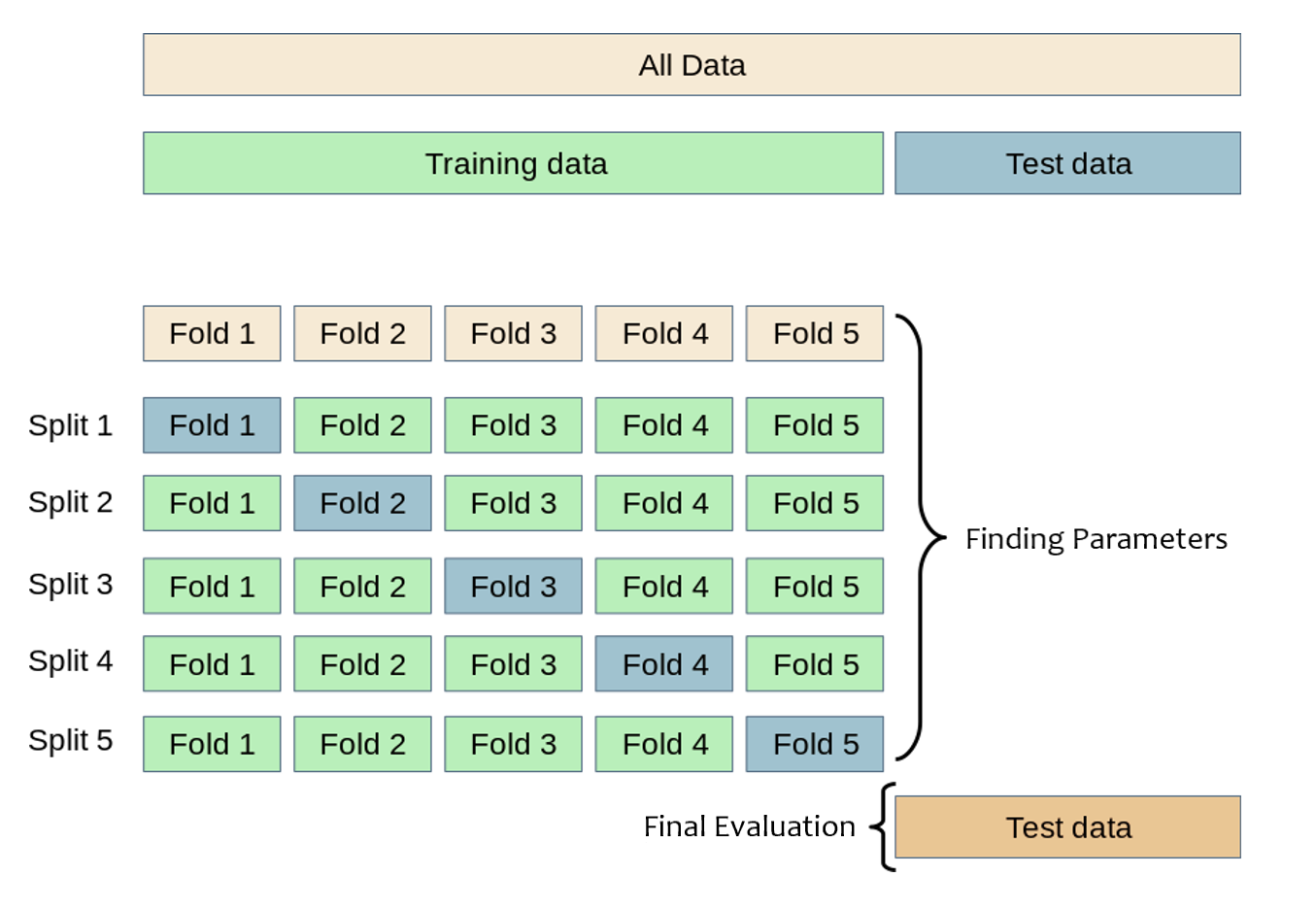
Figure 4.2: Schematic representation of k-fold cross-validation (\(k=5\)). The training set is split into \(k\) smaller sets. The model is trained using \(k-1\) folds and validated on the remaining data. The best model is evaluated in the holdout test set. Modified from scikit documentation.

---

2. RT-DICOM is an extension of the DICOM standard applied to radiation therapy.↩︎

3. Bartlett’s test checks whether a matrix is significantly different from the identity matrix. When applied to a correlation matrix, it provides a statistical probability that there exist significant correlations among at least some of the variables. For factor analysis, some relationships are necessary between variables; therefore, a significant Barlett’s test of sphericity is required, e.g., \(p < 0.001\).↩︎

4. Communality is the proportion of each variable’s variance accounted for by the principal components. Communalities for the \(i_\text{th}\) variable are computed by taking the sum of the squared loadings for that variable, i.e. \(\hat{h}_i^2=\sum_{j=1}^m \hat{\varphi}_{ij}^2\).↩︎

5. LASSO stands for least absolute shrinkage and selection operator.↩︎