3 Literature

3.1 Background

Complexity metrics can be divided into two groups, fluence map-based and aperture-based.²³ The former measure the variations of fluence’s intensity and have originally been described for IMRT plans with multiple static gantry angles. The latter consider MLC openings’ size and shape and can be applied to both IMRT and VMAT plans. For a thorough review, the reader may refer to Hernandez et al²⁴ and Chiavassa et al.²⁵ In this thesis, we study aperture-based metrics.

Various TPSs assign different priorities when modulating the plan parameters. For example, Varian Eclipse plans are demanding for the MLC, rendering them more vulnerable to uncertainties stemming from the use of small apertures and potential errors in the MLC calibration.²⁴ Other TPSs, such as Philips Pinnacle and Elekta Monaco, modulate the gantry speed and the dose rate on top of MLC positions. Therefore, a department’s adoption of a complexity metric should be individualized, considering the differences between treatment planning systems and linear accelerator technical specifications.

3.2 Circumference/Area (CoA)

The ratio of circumference over area may be calculated for each MLC aperture, via the following formula:

\[ \text{CoA}_\text{beam} = \sum_{i=1}^{S} \frac{\text{Perimeter}_i}{\text{Area}_i} \]

where \(S\) is the total number of segments. However, it would be more prudent to take into account the monitor units of the \(i_\text{th}\) segment \((\text{MU}_i)\). Then, the plan’s complexity (\(\text{CoA}_\text{plan}\)) would be written as the sum of CoA over all beams \(B\), weighted by the proportion of MUs delivered through the segments over the total MUs of the plan \((\text{MU}_\text{plan})\):

\[ \text{CoA}_\text{plan} = \frac{1}{\text{MU}_\text{plan}}\sum_{j=1}^B \underbrace{\sum_{i=1}^{S} \frac{\text{Perimeter}_i}{\text{Area}_i} \times \text{MU}_i}_{\text{CoA of }j\text{-th beam}} \]

The advantage of this index is that it conceptually is a straight-forward and tangible metric.²⁰ In Fig. 3.1, the CoA for a patient with locally advanced prostate cancer has been calculated. The plot uses polar coordinates to express complexity as a function of gantry’s rotation. The surge in complexity between \(19\pi/12\) and \(11\pi/6\) exposes the plan to delivery uncertainties, such as intrafraction prostate motion. Ideally, complexity should be spread out over the entire arc. However, this is not always feasible due to the geometric relation of organs at risk and planning treatment volumes.

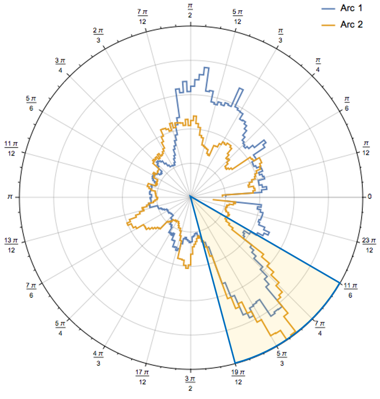
Figure 3.1: Polar plot of complexity (circumference/area) as a function of gantry angle in a patient with locally advanced prostate cancer. The shaded part of the arcs is associated with a high degree of complexity, rendering the plan vulnerable to spatio-temporal uncertainties (e.g., intrafraction prostate motion). Source: Radiation Oncology Department of Papageorgiou General Hospital.

3.3 Leaf Travel (LT)

This index measures the average distance traveled by the moving leaves of the collimator. LT was conceived for VMAT treatments consisting of a single full arc. To allow for straightforward comparisons between plans with different arcs or partial arcs, LT is sometimes divided by the corresponding arc length (typically about 360 degrees for single arcs and about 720 degrees for double arcs). In this thesis, we calculated the plans’ total LT by weighting each arc’s LT based on its monitor units.¹

\[ \text{LT}_{\text{beam}} = \frac{1000(mm) - \text{LT Mean}(mm)}{1000(mm)} \] The plan’s total LT is the weighted sum of beams’ LT over all \(B\) beams:

\[ \text{LT}_{\text{plan}} = \frac{1}{\text{MU}_\text{plan}}\sum_{i=1}^B \text{LT}_\text{beam} \times \text{MU}_i \]

3.4 Edge Metric (EM)

This metric describes the complexity of multileaf collimator apertures based on the ratio of leaf side edge length and the distances between leaves. The constants \(C_1\) and \(C_2\) in the formula below constitute scaling factors that define the relative importance of the \(x\) and \(y\) edges.²⁶ \(A\) is the segment’s area. As the differences between adjacent leaves positions accumulate, the higher the values of EM index are assumed. EM is inherently linked to the tongue-and-groove effect.²⁶ In the original study by Younge et al., the recommended parameters were \(C_1 = 0\) and \(C_2 = 1\) because this combination produced the strongest correlation between EM and the measured dosimetric error. \(W_i\) are the aperture weights that, in their absence, the optimization will be biased towards the regularization of apertures with the lowest number of MUs because any change in these apertures will have the least dosimetric impact.

\[ \text{EM}_\text{beam} = \sum_{i=1}^S W_i \frac{C_1 x_i + C_2 y_i}{A_i} \]

In Fig. 3.2, various segments’ apertures are shown when the edge metric penalty is enabled or disabled in the cost function \(J\). The penalty is recalculated after each iteration during the optimization process and added to the dose-related component of the cost function to yield the total cost. A scaling factor, expressed as the relative importance of EM penalty with respect to the dose-related cost function, is used, i.e. \(J_\text{EM} = \lambda \text{EM}_\text{plan} = \lambda \sum_{i=1}^S W_i y_i/A_i\). In Fig. 3.3, the dose difference between the theoretically calculated and measured doses is shown (\(\lambda = 0.031\)). It is evident how the activation of edge penalty regularizes apertures’ shapes and reduces the dosimetric error.

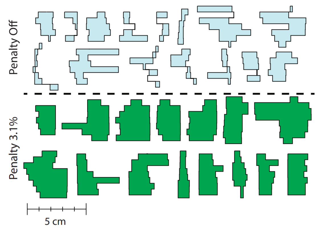
Figure 3.2: Aperture-regularization integration into the objective function of VMAT optimization process. Top: Apertures generated without an edge penalty. Bottom: Apertures generated with an edge penalty. Source: Younge et al.[26}.

Figure 3.3: (a) Dose difference (calculated – measured) in a VMAT plan without the edge penalty. (b) With the edge penalty turned on. (c) Distribution of measured dose deviations. Source: Younge et al.²⁶.

3.5 Equivalent Square Field (ESF) and Mean Field Area (MFA)

ESF is defined as the square root of the total area of the beams’s apperture. In literature, a conversion function, \(f(x) = 1-e^{-x}\), has been used to endow distances with a non-linear contribution to the field’s complexity.²⁰ In this thesis, distances contributed equally to the ESF score. A similar complexity metric is the mean field area, that was found to correlate with gamma passing rates in prostate IMRT plans.^27,28

3.6 Modulation Complexity Score (MCS) and Leaf Travel MCS for VMAT (LTMCSV)

This score considers two contributing factors to a plan’s complexity. Namely, the variability in the shape of beamlets (Leaf Sequence Variability, LSV) and the geometric variation of their aperture area (Aperture Area Variability, AAV).²⁹ The formula for calculating the MCS score of a plan is as following:

\[ \text{MCS}_\text{plan} = \sum_{j=1}^{B} \left[\underbrace{\left(\sum_{i=1}^{S} \text{AAV}_i \times \text{LSV}_i \times \frac{\text{MU}_i}{\text{MU}_{\text{beam,}j}}\right)}_{\text{MCS of } j \text{-th beam}} \times \frac{\text{MU}_{\text{beam,}j}}{\text{MU}_\text{plan}} \right] \]

\[\begin{align*} LSV_j &= \left[\frac{\sum_{i=1}^{N-1} p_\text{max}-(p_i-p_{i+1})}{(N-1) \cdot p_\text{max}}\right]_{\text{left bank},j} \times \left[\frac{\sum_{i=1}^{N-1} p_\text{max}-(p_i-p_{i+1})}{(N-1) \cdot p_\text{max}}\right]_{\text{right bank},j}\\ AAV_j &= \frac{ \sum_{i=1}^N p_{i,_{\text{left bank}}} - p_{i,_{\text{right bank}}}} {N\cdot\left(\text{max}(p_{i,\text{left bank}})-\text{max}(p_{i,\text{right bank}})\right)} \end{align*}\]

where \(p_i\) is the coordinate of the \(i_\text{th}\) leaf position, and \(p_\text{max}\) is the maximum distance between positions for a given leaf bank, summed over all \(B\) beams (arcs) and all segments \(S\) (Fig. 3.4). MCS values range in \([0,1]\), and by the definition above, it follows that the higher the MCS value, the lower the complexity. MCS enables the comparison of complexity between different treatment sites and the comparison of single vs. multiple arcs plans. The largest value of MCS, 1.0, is realized by an open field, since \(p_i = p_{i+1}\):

Figure 3.4: Schematic representation of an aperture’s shape. In both the left and the right banks the extreme right and extreme left leaves are in yellow and red, respectively. The maximum leaf opening, \(p_\text{max}\), corresponds to the the red leaf in the left bank and in the yellow leaf in the right bank. Modified from: Sumida et al.³⁰

\[\begin{align*} LSV_j &= \left[\frac{\sum_{i=1}^{N-1} p_\text{max}}{(N-1) p_\text{max}}\right]_{\text{left bank},j} \left[\frac{\sum_{i=1}^{N-1} p_\text{max}}{(N-1) p_\text{max}}\right]_{\text{right bank},j} = \frac{(N-1) p_\text{max}}{(N-1)p_\text{max}} \frac{(N-1) p_\text{max}}{(N-1)p_\text{max}} = 1\\ AAV_j &= \frac{ \sum_{i=1}^N p_\text{max}} {N p_\text{max}} = 1 \end{align*}\]

Therefore:

\[\begin{align*} \text{MCS}_\text{plan} &=\sum_{j=1}^B \left[\left(\sum_{i=1}^S \frac{\text{MU}_i}{\text{MU}_{\text{beam},_j}}\right) \times \frac{\text{MU}_{\text{beam},_j}}{\text{MU}_\text{plan}} \right] = \sum_{j=1}^B \left[\left(\frac{1}{\text{MU}_{\text{beam},_j}} \sum_{i=1}^S \text{MU}_{i}\right) \times \frac{\text{MU}_{\text{beam},_j}}{\text{MU}_\text{plan}} \right]\\ &=\sum_{j=1}^B \left(\frac{\text{MU}_{\text{beam},_j}}{\text{MU}_{\text{beam},_j}} \times \frac{\text{MU}_{\text{beam},_j}}{\text{MU}_\text{plan}}\right) =\frac{1}{\text{MU}_\text{plan}} \sum_{j=1}^B \text{MU}_{\text{beam},j} = \frac{\text{MU}_\text{plan}}{\text{MU}_\text{plan}} = 1 \end{align*}\]

The original MCS formulation was referring to step and shoot IMRT. However, during a VMAT arc, MUs are delivered in a continuous manner between adjacent control points (CPs). Thus, the calculation of MCS has been slightly modified to adapt to the VMAT case.³¹ Concretely, we must consider the product of the mean values of \(\text{LSV}_i\) and \(\text{AAV}_i\) between adjacent control point:

\[ \text{MCS-VMAT}_\text{beam} = \sum_{i=1}^{S-1}\left( \frac{\text{AAV}_i + \text{AAV}_{i+1}}{2} \times \frac{\text{LSV}_i + \text{LSV}_{i+1}}{2} \times \frac{\text{MU}_{i,i+1}}{\text{MU}_\text{beam}}\right) \]

Although MCS is capable of distinguishing between the levels of complexity of different treatment sites, it has not yet been validated as a surrogate marker of dosimetric deviations for specific treatment sites. A multiplicative combination of mean leaf travel and modulation complexity score has also been proposed, i.e. \(\text{LTMCS} = \text{LT} \times \text{MCS}\),³¹ or \(\text{LTMCSV} = \text{LT} \times \text{MCSV}\) for the case of a VMAT plan.

3.7 Modulation Index total (\(\text{MI}_\text{total}\))

This index involves the variations in speed and acceleration of the MLC, as well as variations of the gantry speed (GA) and the dose rate (DRV).³² Its calculation is based on the concept of Modulation Index introduced by Webb.³³ First, we define a “counting” function \(z_\text{total}(f)\):

\[\begin{align*} z_\text{total}(f) &=\frac{1}{S-2} \sum_{i=1}^{S} \bigg[N_i\Big( \text{MLC speed}_i>f \sigma_{\text{MLC speed}} \text{ or } \text{MLC accel}_i > \alpha f \sigma_{\text{MLC}_\text{accel}} \Big) \\ &\cdot W_{\text{GA},i+1} \cdot W_{\text{MU},i+1}\bigg] \end{align*}\]

where \(S\) is the total number of control points and:

\[N_i\Big( \text{MLC speed}_i>f \sigma_{\text{MLC speed}} \text{ or } \text{MLC accel}_i > \alpha f \sigma_{\text{MLC}_\text{accel}}\Big)\]

means that if the MLC speed or acceleration at the \(i_\text{th}\) control point is larger than \(f\sigma_{\text{MLC speed}}\) or \(\alpha f \sigma_{\text{MLC}_\text{accel}}\), respectively, then the value of that CP becomes \(1\) multiplied by the weight factors \(W_{\text{GA},i+1}\) and \(W_{\text{MU},i+1}\), \(\sigma_{\text{MLC speed}_i}, \sigma_{\text{MLC accel}_i}\) being the standard deviations of MLC \(\text{speed}_i\) and MLC \(\text{accel}_i\), respectively. The \(f\) argument controls therefore the “threshold” beyond which a leaf pair contributes to complexity, and, similarly, \(\alpha\) is a scaling factor that empirically is set to \(\alpha = 1/\text{Time}_i\). The weight factors are defined by the following formulas:

\[\begin{align*} {}&W_{\text{GA,}_{i+1}} = \frac{\beta}{1+(\beta-1)\exp\left(-\frac{\text{GA}_i}{\gamma}\right)}\\ {}&W_{\text{MU,}_{i+1}} = \frac{\beta}{1+(\beta-1)\exp\left(-\frac{\text{DRV}_i}{\gamma}\right)} \end{align*}\]

In the paper of Park et al.³² it is \(\beta = \gamma = 2\), and the gantry acceleration \(\text{GA}_i\) and dose rate variation \((\text{DRV}_i)\) are calculated as:

\[\begin{align*} \text{GA}_i &= \left| \frac{\Delta\text{Gantry angle}_i}{\text{Time}_i} - \frac{\Delta\text{Gantry angle}_{i+1}}{\text{Time}_{i+1}} \right|\\ \text{DRV}_i &= \left|\text{DR}_i - \text{DR}_{i+1}\right| \end{align*}\]

Finally, \(\text{MI}_\text{total}\) is calculated as the sum of the contributions of all the individual leaves:

\[ \text{MI}_t = \sum_{i=1}^{N_\text{leaves}} \int_0^k z_\text{total}(f)\mathrm{d}f, \hspace{1cm} k = 0.2, 0.5, 1 \text{ and } 2 \]

3.8 Plan Irregularity (PI)

PI quantifies the deviations of aperture shapes from a circle,²³ with \(\text{PI}=1\) corresponding to a perfect circle. In Fig. 3.5 aperture area (AA) of beam \(b\) and segment \(s\) is given by:

\[ \text{AA}_{bs} = \sum_{k=1}^{N_{\small\text{LP}}} t_k\left(x_{bsk}^{(2)} - x_{bsk}^{(1)}\right) \]

Where \(k\) is the leaf pair index, \(N_\text{LP}\) is the total number of leaf pairs, \(t_k\) is the width of the \(k_\text{th}\) leaf pair and \(x^{(1)}, x^{(2)}\) are the positions of the leaves of te pair. The aperture irregularity is computed as:

\[ \text{AI}_{bs} = \frac{\text{AP}_{bs}^2}{4\pi \text{AA}_{bs}} \]

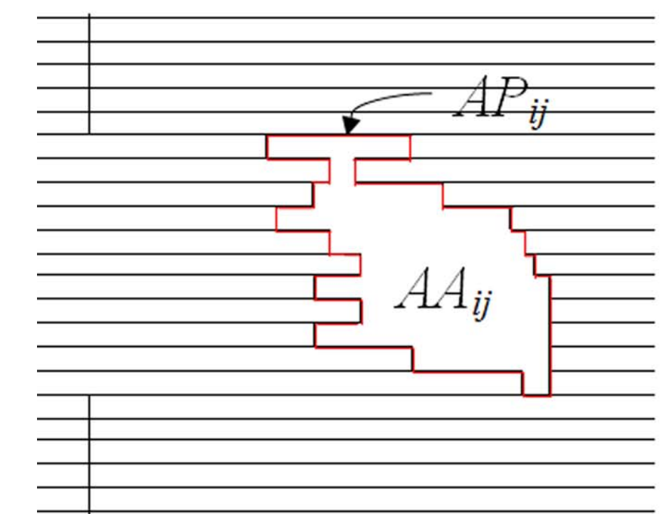
Figure 3.5: Schematic representation of beam aperture analysis for the plan irregularity index.

For instance, for a square segment \(\text{AP} = 4a, \text{AA} = a^2\). Then:

\[ \text{AI}_{bs} = \frac{16a^2}{4\pi a^2} = \frac{4}{\pi} \simeq 1.273 \]

On the contrary, for a perfect circular segment it holds that \(\text{AP} = 2\pi R, \text{AA} = \pi R^2\). Then:

\[ \text{AI}_{bs} = \frac{4\pi^2 R^2}{4\pi \cdot\pi R^2} = 1 \]

Given the quantities above one can define beam irregularity (BI) of beam \(b\) averaged over all \(S\) segments:

\[ \text{BI}_{b} = \frac{\sum_{s=1}^S\text{MU}_{bs} \text{AI}_{bs}}{\text{MU}_{b}} \]

And the plan irregularity (PI) averaged over all \(B\) beams:

\[ \text{PI} = \frac{\sum_{b=1}^B\text{MU}_{b} \text{BI}_{b}}{\text{MU}_{\text{plan}}} \]

3.9 Small Aperture Score (SAS)

The small aperture score (SAS) is defined as the ratio of open leaves for which the aperture is less than a predefined threshold (e.g., 2, 5, 10mm) to all open leaf pairs:

\[ \text{SAS}(x)_{\text{beam}} =\sum_{i=1}^S \left[\frac{N(x>a>0)_i}{N(a>0)_i} \times \frac{\text{MU}_i}{\text{MU}_\text{beam}}\right] \]

Where \(x\) is the aperture criteria, e.g., \(x = \{2, 5, 10\}\), \(S\) is the number of segments in the beam, \(N\) is the number of leaf pairs not blocked by the jaws, and \(a\) is the aperture distance between opposing leaves. The \(\text{SAS}(5\text{mm})\) metric has been found to correlate well with \(\Gamma(2\%/2\text{mm})\) pass rates.²⁷ Also, \(\text{SAS}(5\text{mm})\) was able to provide a threshold below which all plans passed their MapCHECK diode array QA tests, and above which only a small percentage of verified plans were identified, incorrectly, as likely to fail the QA process.

---

1. There were no plans with partial arcs in our dataset.↩︎